http://dx.doi.org/10.4236/am.2014.53050
Study of Delay and Loss Behavior of Internet
Switch-Markovian Modelling Using Circulant
Markov Modulated Poisson Process (CMMPP)
Ranadheer Donthi1, Ramesh Renikunta2, Rajaiah Dasari3, Malla Reddy Perati3
1
Department of Mathematics, Medak College of Engineering and Technolgy, Medak, India
2
Department of Mathematics, Kakatiya Institute of Technology and Science, Warangal, India
3
Department of Mathematics, Kakatiya University, Warangal, India Email: [email protected], [email protected],
[email protected], [email protected]
Received September 29, 2013; revised October 29, 2013; accepted November 7, 2013
Copyright © 2014 Ranadheer Donthi et al. This is an open access article distributed under the Creative Commons Attribution Li-cense, which permits unrestricted use, distribution, and reproduction in any medium, provided the original work is properly cited. In accordance of the Creative Commons Attribution License all Copyrights © 2014 are reserved for SCIRP and the owner of the intel-lectual property Ranadheer Donthi et al. All Copyright © 2014 are guarded by law and by SCIRP as a guardian.
ABSTRACT
Most of the classical self-similar traffic models are asymptotic in nature. Therefore, it is crucial for an appropri-ate buffer design of a switch and queuing based performance evaluation. In this paper, we investigappropri-ate delay and loss behavior of the switch under self-similar fixed length packet traffic by modeling it as CMMPP/D/1 and
CMMPP/D/1/K, respectively, where Circulant Markov Modulated Poisson Process (CMMPP) is fitted by
equat-ing the variance of CMMPP and that of self-similar traffic. CMMPP model is already the validated one to emu-late the self-similar characteristics. We compare the analytical results with the simulation ones.
KEYWORDS
CMMPP; Self-Similar Traffic; Mean Waiting Time; Packet Loss Probability; Traffic Intensity; Hurst Parameter; Time-Scale
1. Introduction
position of several 2-state Interrupted Poisson Processes (IPPs). The said models hold well for voice traffic as IPP consists of two states talkspurt and silence. On the other hand, the Circulant Markov Modulated Poisson Process (CMMPP) is a Poisson process, the rate of which is changed according to circulant Markov chain [8]. The Circulant Markov Modulated Poisson Process is characterized by circulant stochastic transition matrix Q and non-negative vector λ. In the case of two states Circulant Markov Modulated Poisson Process (2-CMMPP) which is Switched Poisson process (2-state MMPP), two states are active unlike IPP and it is good model for ar- rival process in Internet traffic. The MMPP and CMMPP both are model classes which can be incorporated in queuing analysis. The CMMPP has several advantages over MMPP in terms of computational complexity [9,10]. The steady state probability distributions of this process are the normalized null vector of its generator matrix.
In addition to traditional data services, multimedia and real-time applications are becoming indispensable ser- vices offered by the best-effort Internet. The future Internet is expected to offer a certain QoS guarantee to some important applications, which are the best effort today. As is well understood, packets may suffer some delay and loss at the network nodes during their traversal across a packet-switched network. Therefore, packet loss and end-to-end delay are two crucial performance metrics for Internet QoS. In the present paper, we investigate delay and loss behavior of the resultant CMMPP/D/1/K queueing system and compare with that of simulation results.
The paper is organized as follows. In Section 2, we first overview the fundamentals of self-similar process and Circulant Markov modulated Poisson process. In Section 3, the generalized fitting procedure is given. In Sec- tion 4, Queuing systems and numerical results are presented. Finally, some conclusions are made in Section 5.
2. Self-Similar Process and Circulant Markov Modulated Poisson Process (CMMPP)
In this section, we first overview the definition of the exact second order self-similar process and summarize some characteristics of CMMPP and then, we make some remarks.
2.1. Self-Similar Process
The definition of exact second-order self-similar processes is given as follows. If we consider X as a second -order stationary process with variance σ2, and divide time axis into disjoint intervals of unit length, we could define X =
{
X tt =1, 2, 3.}
to be the number of points (packet arrivals) in theth
t interval. A new sequence
( )m
{ }
( )m , tX = X where ( ) ( )1
1
1
, 1, 2, 3,
m m
t t m i
i
X X t
m = − +
=
∑
= , is the average of the original sequence in m non-overlapping blocks. Then the process X is defined as an exact second order self-similar process with the Hurst parameter, H = −1 β 2, if
( )
( )
2Var X m =σ m−β,∀ ≥m 1. (1)
2.2. Circulant Markov Modulated Poisson Process (CMMPP)
CMMPP is a doubly stochastic process in which arrival rate is given by λ
[ ]
Jt , where J tt, ≥0 is anm
-stateMarkov process. The arrival rate can therefore take on only m values, namely λ λ1, 2,,λm. It is equal to λj
whenever the Markov process is in the state ,1j ≤ ≤j m. The CMMPP is fully parameterized by the infinitesimal generator Q (Circulant Markovian) of the Markov process and the vector λ=
(
λ λ1, 2,,λm)
of the arrival rates.Let Λ be the diagonal matrix with Λ =jj λj,1≤ ≤j m. In the case of two state CMMPP, Q and Λ are given as follows:
1 1 1
1 1 2
0
, .
0
c c
Q
c c
λ λ
−
= Λ =
−
(2)
The mean and variance of Nt can be deduced from that of MMPP [7]. The mean arrival rate λ of CMMPP is
given by λ= Λπ e, where π is the stationary probability vector of Q, i.e. πQ=0,πe=1 and e is an all 1
column vector with designated dimension. If we let Nt, t≥0, be the number of arrivals in (0, t],
The mean,
( )
1 2 .2
t
E N =λ λ+ t (3)
[ ]
(
)
(
)
12 2
1 2 1 2 2
1 2
2
1 1
Var 1 e
2 4 8
c t t
N t t
c c
λ λ λ λ
λ λ+ − − −
= + − − (4)
Since the index of dispersion for counts (IDC) is defined as
( )
Var[ ]
[ ]
t tN IDC t
E N
=
From (3) and (4), we can obtain
( )
(
(
)
)
(
)
(
)
(
)
1 2 2 2 1 2 1 2 21 1 2 1 1 2
1 e 1
2 4
c t
IDC t
c c t
λ λ λ λ
λ λ λ λ
−
− −
−
= + −
+ + (5)
We then could obtain the following remarks:
1) IDC t
( )
→1, as t→0 , that is, CMMPP tends to a Poisson process.2)
( )
(
)
(
)
2 1 2
1 1 2
1 , 2 IDC t c λ λ λ λ − → +
+ a constant , as t→ ∞.
3) IDC t
( )
is monotonic increasing over a finite time interval and is bounded. 4) Steady state distribution of 2-state CMMPP is 1 1,2 2
and is independent of transition rates.
The first and second order statistics of Nt in the case of MMPP and CMMPP are listed in the following table.
Measures MMPP CMMPP
Mean ( ) 2 1 1 2 1 2 t
c c E N t
c c
λ+ λ =
+ E N( )t 12 2t.
λ λ+ =
Variance
[ ] ( ) ( )
( )
( )
( ) (1 2)
2 1 2 1 2
3 1 2 2
1 2 1 2 4 1 2 2 Var 2 1 e t t
c c t
c c
N E N t
c c c c
c c
λ λ
λ λ +
− = + + − − − + [ ] ( )
( ) 1
2 1 2 1 2 1 2 2 1 2 2 1 Var 2 4 1 e 8 t t c t
N N t t
c
c
λ λ λ λ
λ λ −
− + = + − − − IDC ( ) ( ) ( ) ( ) ( )
( ) ( ) (1 2)
2 1 2 1 2
2
1 2 2 1 1 2
2 1 2 1 2
3
1 2 2 1 1 2
2 1
2
1 e cc t
c c IDC t
c c c c c c
c c c c t
λ λ λ λ λ λ λ λ − + − = + + + − − − + +
( ) ( ( )2) ( ()2
(
)21)
1 21 2
2
1 1 2 1 1 2
1 e 1
2 4
c t
IDC t
c c t
λ λ λ λ
λ λ λ λ
−
− − −
= + −
+ +
3. Generalized Variance Based Fitting Procedure
Generalized variance-based fitting method is a procedure to find out the traffic model parameters, that match the variance of self-similar and that of model traffic [4-6,11]. The fitted model emulating self-similar traffic consists of a superposition of d' 2-CMMPPs and one Poisson process. We describe the ith 2-CMMPP as follows.
1 2
0
, .
0
i i i
i i
i i i
c c Q c c λ λ − = ∧ = −
(6)
Superposition of above ' 'd CMMPPs and a Poisson process is a transition rate matrix and is determined by
1 2 d, 1 2 d p
Q=Q ⊕Q ⊕ ⊕ Q ∧ = ∧ ⊕ ∧ ⊕ ⊕ ∧ ⊕ λ (7)
In (7), ⊕ means the Kroneker’s sum and λp is the arrival rate of the Poisson process. The whole arrival
rate, λ, is then given by
1 2 1 . 2 d i i p i λ λ λ λ = +
= +
∑
(8)Let Nt i,,Nt p, be the number of arrival packets from the ith CMMPP and Poisson process, respectively, dur-
ing the tth time slot, and let ( ), m t i
N and ( ), m t p
CMMPP and Poisson process, respectively. Put ( ) ( ) ( ) , , 1 . d
m m m
t t i t p
i
X N N
=
=
∑
+ (9)Using (4), we obtain the variance of the ith CMMPP as
( )
( )
1 2(
2)
(
)
2, 2 2 1 2
1 1
Var 1 e
2 4 8
i
m i i mc
t i i i
i i
N
m mc m c
λ +λ − λ λ
= + − − −
(10)
Also
( )
( )
,Var Nt pm p
m λ
= . (11)
From (9)-(11) and using the fact that superposition of independent sub-processes preserves the variance, we obtain
( )
1 2(
)
21 2 1 1 Var , 2 d d p
m i i
t i i i
i i
X
m m
λ λ λ η λ λ
= =
+
= +
∑
+∑
− (12)where
(
2)
2 2
1 1
1 e .
4 8
i mc i
i
mci m c
η = − − −
(13)
Using (1) and (12), we can match the variance at ' 'd different points mi, i=1, 2, 3,, .d Let
[
mmin,mmax]
(
mmin ≤ ≤m mmax)
be the time interval over which we want the process to express self-similarity of the originalprocess, then mi is given by
1
min , 1, 2, 3, , , i
i
m =m a− i= d (14)
where 1 1 max min , 1. d m a d m −
= >
(15)
Now, we assume the following relations between ci and mi
(
1)
.i i
m c =const ≤ ≤i d
That is, ci can be determined using
1
1, 1, 2, , . i
i
m
c c i d
m
= = (16)
There are due to the fact that a Self-similar process takes the same in any time scale. Because of this assump-tion, we can reduce the number of parameters to be determined. That is, if we determine ci, we can obtain the
values of ci
(
2≤ ≤i d)
by using (16). Furthermore, we can obtain λp from (8) if we determine λ λ1i, 2i. Theparameters we need to find are only ci,λ1i and λ2i.
4. Queuing Systems and Numerical Results
In this section, synchronous input traffic of fixed length h (in time units) is modeled as CMMPP/D/1queuing system. In CMMPP/D/1 system, the packets of fixed length arrive according to CMMPP. The performance me-trics in this case involve m m× irreducible matrix G=
( )
Gij if CMMPP of m states [12], where Gij is theprobability that a busy period starting with the CMMPP in state i and ends in state .j The matrix G is a key ingredient in obtaining mean waiting time. The mean waiting time (MWT) could be computed by the formula [11].
(
1)
2 ( )2 2(
(
1)
)
(
)
12 1 tot
MWT ρ h λ h ρ g hπ Q eπ λ
ρ
−
= + − − + Λ +
− (17)
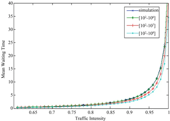
The steady state vector g of G satisfies gG=g ge, =1. For the packet loss probability, the switch is modelled as finite buffer queueing system CMMPP/D/1/K [6,12]. Packet loss probability against traffic intensity is com- puted using the procedure [6,12]. We have fitted CMMPPs for the traffic parameters H = 0.7, H = 0.8, H = 0.9, λ = 1, σ2 = 0.6 over the time scales [102, 106] [102, 107] [102, 108]. In all the above cases, the number of two state CMMPPs, d, is equal to 4. Numerical calculations are performed using the MATLAB and the results are shown in the Figures 1-6. Figure 1 depicts the mean waiting time against traffic intensity for the case of H = 0.7 and the different time scales [102, 106], [102, 107] and [102, 108]. In this case, analytical results are validated with that of simulation. From this figure, it is clear that, the mean waiting time increases as the traffic intensity increases.
Figure 2 depicts the mean waiting time against the traffic intensity for the case H = 0.8, and the time scales [102,
106], [102, 107], and [102, 108]. From the figure, it is clear that mean waiting time decreases as the time increases.
Figure 3 depicts the mean waiting time against the traffic intensities for the case H = 0.7, H = 0.8, H = 0.9, over
the time scale [102, 108]. From this we infer that the mean waiting time increases as H increases. Figure 4de- picts the packet loss probability against the traffic intensity for the case of H = 0.8 over the time scales [102, 106], [102, 107], and [102, 108]. From this figure, we conclude that packet loss probability increases as the traffic in- tensity increases. Figures 5-6 depict the packet loss probability against the traffic intensitiesfor the cases of H =
[image:5.595.167.462.516.719.2]Figure 1. Mean waiting time of the resultant CMMPP/D/1 queue with d = 4, H = 0.7, λ = 1, σ2 = 0.6.
Figure 3. Mean waiting time of the resultant CMMPP/D/1 queue with d = 4, λ = 1, σ2 = 0.6 over the time scale [102, 108].
Figure 4. Loss probability of the resultant CMMPP/D/1/K queues with d = 4, λ = 1, H = 0.8, and K = 10.
Figure 5. Loss probability of the resultant CMMPP/D/1/K queues with d = 4, λ = 1, and K = 10 over the time scale [102,
[image:6.595.169.462.520.707.2]Figure 6. Loss probability of the resultant CMMPP/D/1/K queues with d = 4, λ = 1, and K = 10 over [102, 107].
0.7, H = 0.8, H = 0.9, over the time scales [102, 106], and [102, 107], respectively. From these figures, we con- clude that packet loss probability decreases as the time scale increases, and packet loss probability decreases as the Hurst parameter decreases.
5. Conclusion
Most of the parsimonious self-similar traffic models proposed earlier are asymptotic in nature, therefore, they are less effective in the context of queuing based performance evaluation. Markovian models emulating self- similar traffic are proposed, as they hold well for queueing theory. These models are based on second order sta-tistics. In this paper, we investigated queuing delay and loss behavior over different time scales and for different Hurst parameters. It is found from the numerical results that self-similar can be well represented by the proposed model. Our numerical results reveal that time-scale does have impact on packet loss probability. Packet loss probability increases as H and ρ increase. Based on the analysis presented in this paper, one could select the ap-propriate time-scale in the generalized variance based fitting method to meet the QoS requirement. This kind of analysis is useful in dimensioning the switch under self-similar input traffic.
REFERENCES
[1] W. E. Leland, M. S. Taqqu, W. Willinger and W. V. Wilson, “On the Self-Similar Nature of Ethernet Traffic (Extended Ver-sion),” IEEE/ACM Transactions on Networking, Vol. 2, No. 1, 1994, pp. 1-15. http://dx.doi.org/10.1109/90.282603
[2] V. Paxson and S. Floyd, “Wide Area Traffic: The Failure of Poisson Modelling,” IEEE/ACM Transactions on Networking, Vol. 3, No. 3, 1995, pp. 226-244. http://dx.doi.org/10.1109/90.392383
[3] M. Crovella and A. Bestavros, “Self-Similarity in World Wide Web Traffic: Evidence and Possible Causes,” IEEE/ACM Transactions on Networking, Vol. 5, No. 6, 1997, pp. 835-846. http://dx.doi.org/10.1109/90.650143
[4] A. Andersen and B. Nielsen, “A Markovian Approach for Modeling Packet Traffic with Long-Range Dependence,” IEEE Journal on Selected Areas in Communications, Vol. 16, No. 5, 1998, pp. 719-773. http://dx.doi.org/10.1109/49.700908
[5] T. Yoshihara, S. Kasahara and Y. Takahashi, “Practical Time-Scale Fitting of Self-Similar Traffic With Markov Modulated Poisson Process,”Telecommunication Systems, Vol. 17, No. 1-2, 2001, pp. 185-211.
http://dx.doi.org/10.1023/A:1016616406118
[6] S. Kasahara, “Internet Traffic Modelling: Markovian Approach to Self-Similar Traffic and Prediction of Loss Probability for Finite Queues,” IEICE Transactions on Communication Special Issue on Internet Technology, Vol. E84-B, No. 8, 2001, pp. 2134-2141.
[7] S. K. Shao, P. Malla Reddy, M. G. Tsai, H. W. Tsao and J. Wu, “Generalized Variance-Based Markovian Fitting for Self-Sim- ilar Traffic Modeling,” IEICE Transactions on Communication, Vol. E88-B, No. 12, 2005, pp. 4659-4663.
[9] K. De Cock, T. Van Gestel and B. De Moo, “Identification of Circulant Modulated Poisson Process a Time Domain Approach,” Proceedings of MTNS, 1998, pp. 739-742.
[10] C. Blondia, “The N/G/l Finite Capacity Queue,” Communications in Statistics: Stochastic Models, Vol. 5, 1989, pp. 273-294.
[11] D. Ranadheer, R. Ramesh, D. Rajaiah and P. Malla Reddy, “Self-Similar Network Traffic Modeling Using Circulant Markov Modulated Poisson Process (CMMPP) (Manuscript),” Communicated to International Conference on Fractals and Wavelets, 2013.
![Figure 3. Mean waiting time of the resultant CMMPP/D/1 queue with 10d = 4, λ = 1, σ2 = 0.6 over the time scale [102, 8]](https://thumb-us.123doks.com/thumbv2/123dok_us/7991453.759530/6.595.169.462.520.707/figure-mean-waiting-time-resultant-cmmpp-queue-scale.webp)
![Figure 6. Loss probability of the resultant CMMPP/D/1/K queues with d = 4, λ = 1, and K = 10 over [102, 107]](https://thumb-us.123doks.com/thumbv2/123dok_us/7991453.759530/7.595.156.473.85.280/figure-loss-probability-resultant-cmmpp-d-k-queues.webp)
