Munich Personal RePEc Archive
Equity Basis Selection in Allocation
Environments
Aadland, David and Kolpin, Van
University of Wyoming, University of Oregon
1 March 2008
Online at
https://mpra.ub.uni-muenchen.de/8725/
E
QUITYB
ASISS
ELECTION INA
LLOCATIONE
NVIRONMENTSAbstract. The successful formation and long-term stability of a cooperative venture is often linked to the perceived fairness of the associated cost or resource allocation. In particular, the effectiveness of such collaborations can be hampered by the lack of a consensus view on what basis should be used for gauging an allocation’s “fairness.” Standards of equity in traditional cost-sharing applications could be assessed on many dimensions: per capita, per unit of demand, or per unit of revenue, to mention a few. This multiplicity of logically compelling “equity bases” is a feature common to many practical cost-sharing applications. Our analysis shows that
features of the allocation environment are capable of explaining a substantial amount of the variation in the equity bases employed in practice and are consistent with the axiomatic principles of collective behavior.
JEL classification numbers: C71, D63, C25
Key words: cooperative games, cost allocation, equity, probit model
David Aadland and Van Kolpin†∗
Department of Economics and Finance Department of Economics 1000 E. University Avenue 1285 University of Oregon Laramie, WY 82072 Eugene, OR 97403-1285 [email protected] [email protected]
† We thank Marty Van Cleave, Bob Hill, Jim Kindle, Rick Krannich, Stephanie Kuster, and, of course, our survey
respondents.
1
1. Introduction
Successful formation and long-term stability of a cooperative venture are often linked to the
perceived fairness of the associated cost or resource allocation. Whether a venture is a simple
business partnership or a global collaboration, such as that which led to the Kyoto protocol, its
effectiveness can be hampered by the lack of a consensus view on what basis should be used for
gauging an allocation’s “fairness.” Consider, for instance, the classic airport problem in which
multiple airlines share a common landing strip (Littlechild and Owen, 1973). Aside from the
issue of how costs should be apportioned amongst the set of players is the more fundamental
question of what represents the relevant basis over which principles of equity should be applied.
Should concern be focused on the distribution of costs across the set of airlines, the set of flights,
the set of passengers, the set of revenues, or perhaps some other basis? Although these various
bases are intertwined, each offers a different perspective on notions of fair treatment. This
multiplicity of logically compelling fairness bases is a feature that is common to many practical
cost-sharing applications. For example, participants of international initiatives to mitigate
global climate change must agree whether the burden of reducing greenhouse gases should be
distributed according to a per capita, per unit of GDP, per unit of wealth, or some other basis
(Ashton and Wang, 2003).1 What then leads to the selection of one basis over another in
practice? Is this choice essentially arbitrary or can parameters of the cooperative environment
predict the fairness basis that is embraced? Moreover, if such explanatory power exists, is it
consistent with theoretical principles of collective behavior? This paper aims to shed light on
these puzzles.
1 The issue of the appropriate equity basis has become a major obstacle to the effective implementation of
2
Much of the theoretical cost-sharing literature employs axiomatic principles to derive a
unique cost-sharing rule. This methodology operates under the premise that a collective decision
on which allocation rule to employ should depend solely on the mathematical structure of the
associated cost-sharing game. While this has proven to be a useful theoretical approach,
practical applications often involve a variety of distinct fairness bases, even when their
associated cost-sharing games are indistinguishable. We introduce the benefit inequity principle
which posits that the greater the differences in benefits realized by elements of a given equity
basis, the greater the pressure to adopt an alternative basis. Our empirical analysis will test the
efficacy of this axiom as a guiding force in the selection of actual cost-sharing procedures.
We use irrigation cost sharing in two neighboring counties of Montana, USA as a context for
our study. The context is well suited for our study, thanks in part to the close geographic and
social proximity of the sample. This closeness makes it less likely that unobserved variation in
cultural conventions, which may in turn influence cooperative decision making, will bias our
estimates. Another compelling feature of our data is that the cost-sharing practices observed on
these ditches are long-lived, in many cases over a century old. Although disputes between
individual ranchers do arise on occasion, the cost-allocation practices have proven to be
remarkably stable.
The ditches in our sample share a common physical structure. The “main” ditch begins at the
headgate, which diverts water from the source stream, and continues in a sequential path through
the users’ properties. Costs for private ditches that branch off the main ditch are covered by their
respective owners and are not shared by the group as a whole. Examples of shared costs include
3
The ditches are used to irrigate hay fields and other cash crops, water livestock, and irrigate
lawns and gardens, with some variation in these uses across the ditches.
Our data set is constructed from a combination of state and federal sources, as well as our
own survey efforts. The data strongly support the conclusion that the benefit inequity principle
serves as a guiding force in the selection of an actual equity basis. In particular, the coefficients
of our empirical model have signs consistent with this principle and our independent variables
exhibit considerable explanatory power.
2. Axiomatic Motivation
Much of the theoretical cost-sharing literature adopts essentially the same methodology as
that pursued in the creation of the bargaining solution (Nash, 1950) or the Shapley value
(Shapley, 1953). In loose terms, this methodology formulates a mathematical abstraction of the
universe of all environments under consideration, identifies desirable properties of a “solution”
defined on this universe, and then demonstrates that these properties will in fact characterize a
unique solution or class of solutions. For instance, the “Shapley program” considers the universe
of all TU (transferable utility) games, defines a solution as a value operator, and then
demonstrates that the Shapley value is the only solution to satisfy the anonymity, additivity, and
dummy axioms.
The approach adopted in our paper differs from that outlined above in several important
respects. First, each irrigation ditch in our universe of cost-sharing environments has not one,
but three distinct “populations” that can serve as the “player” set over which equity is assessed –
namely, the population of irrigators using the ditch, the population of acres irrigated by the ditch,
4
a share of stock ownership of the ditch.) As each of these populations provides a different basis
for equity assessment, we shall refer to these populations generally as equity bases, and
specifically as the per capita basis, per acre basis, and per water-share basis respectively.2
Recall, the focus of our paper is to investigate whether features of the cost-sharing environment
are able to explain the selection of the equity basis used in practice.
A second dimension where our approach differs from traditional treatments of cost sharing is
that we consider the possibility that features of the cost-sharing environment, in particular ones
that have absolutely no effect on the values subject to redistribution, may influence the choice of
allocation procedure. In our setting, ditch maintenance costs are the only values subject to
redistribution. A traditional approach would dictate that the universe of cost-sharing games
should be expressed in terms of only those parameters that impact the costs to be shared and the
player population over which sharing is to occur. We depart from the traditional approach and
hypothesize that the benefits accruing across the ditch may influence the equity basis embraced
even though these benefits are not themselves subject to redistribution.
A final dimension of difference in our approach is that we do not to use axiomatic principles
to identify a unique cost-sharing rule that should be employed. Instead, we seek to examine
whether axiomatic principles are consistent with how features of the cost-sharing environment
determine the equity bases that are employed.
The irrigation cost-sharing environments under consideration are characterized by the
maintenance costs incurred on the ditch, the population of users that have access to the ditch (the
user basis), the population of acres serviced by the ditch (the acre basis), the population of water
shares distributed across users of the ditch (the water-share basis), and the benefits that accrue to
2 In principle, additional equity bases could also be considered. As we were unable to detect the use of alternative
5
ditch users. A comprehensive description of cost sharing on an irrigation ditch would detail the
determining factors of which equity basis is selected as well as the manner in which the costs of
each individual maintenance project are allocated. As our focus is solely on the question of how
equity bases are determined, we will forego any detailed discussion of how costs are distributed
across a given equity basis, e.g., serial versus average cost sharing. The interested reader can
turn to Aadland and Kolpin (2004) for a treatment of this latter subject.
A key axiom underlying our analysis is that of the benefit inequity principle. The essential
idea behind this principle is that since only costs (not benefits) are subject to redistribution, there
may be a fundamental pressure to administer cost sharing over a “level playing field.” That is,
greater pre-tax benefit inequity from the perspective of a given equity basis may imply a
diminished commitment to use that basis to administer costs and assess fairness.
Benefit inequity principle: Greater differences in the irrigation benefits realized by elements of
a given equity basis imply greater pressure to adopt an alternative equity basis.
The reader will note that our formulation of the benefit inequity principle does not delineate
when inequity pressures reach the point where one equity basis will be chosen over all others.
Similarly, the principle does not impose a precise specification for how the benefit differences
across an equity basis are to be measured, e.g., by sample variance, Gini coefficient, maximum
realized benefit minus minimum realized benefit, or some other statistical measure. This
vagueness enables our data to speak to where these lines should be drawn, rather than having
6
3. The Data
The cost-sharing agreements within our sample represent a set of stable, yet informal
conventions that are “understood” by the ditch users. As these conventions are not documented
in publicly available sources, we surveyed the users to obtain information regarding their
cost-sharing procedures and the circumstances surrounding their use. Our survey efforts revealed that
there are three bases over which costs are shared in our sample. Costs are either shared on a per
capita basis, a per acre basis, or a per water-share basis. (Our survey also delved into the issue of
whether the group who shares responsibility for costs may differ depending on the nature of the
project that induced the costs, the subject of which was the focus of Aadland and Kolpin, 2004.
Our focus in the present paper is instead on the determination of an appropriate equity basis.)
Our survey yielded a total of 270 usable responses from 101 of the 169 irrigation ditches in
Carbon and Stillwater counties. These ditches service 2,840 individual parcels of irrigated land,
comprising a total of 150,000 acres. Three ditches were excluded from the analysis because
there was only one reported user and therefore no need for cost sharing. An additional 14 ditches
were excluded because the respondents either (a) reported no cost sharing or (b) they did not
select any of the cost-sharing options in the survey, instead choosing “Other” without specifying
in their written comments how costs were actually shared. Our final sample therefore includes
84 ditches that can be associated with either a per capita, per acre, or per water-share rule.
As might be expected given the informal nature of the cost-sharing arrangements, the
reported rules were not always consistent across users. Apparent inconsistencies in the stated
cost-sharing rule were resolved by assigning to each ditch the rule stated by the majority of its
respondents and, if a tie were to occur (there were seven ties) the most common rule in the
7
In addition to our survey, we relied on several other sources to construct our data set. First,
the Water Resource Division of the Montana Department of Natural Resources and Conservation
(DNRC) provided information on the location and size for the parcels of land serviced by the
irrigation ditches in our sample, as well as the primary use3 for the water (Water Resource
Division, 2002). Second, we used the Soil Surveys for Carbon and Stillwater counties (USDA,
1975 and 1980) to derive estimates of the irrigated and non-irrigated productivity of the land
served by a ditch. These estimates were in turn used to formulate a measure of the benefits
bestowed by access to the irrigation ditch. Finally, we use spatial climate maps produced by the
Oregon Climate Service to generate measures of expected rainfall along the ditches in our
sample, another factor impacting the incremental benefits of irrigation (Oregon Climate Service,
2002).
We now turn to the specification of the variables used in our econometric analysis. Because
we only consider three equity bases (i.e., per capita, per acre, and per water-share), it suffices to
consider two dependent variables – PC and PA. PC is a ditch-level binary variable that is equal
to one if costs are shared on a per capita basis and zero if an alternative basis is employed.
Similarly, PA is a ditch-level binary variable that equals one if costs are shared on a per acre
basis and zero otherwise. Given that there are three bases that appear in our sample, it follows
that if PC=PA=0, then costs are distributed on a per water-share basis.
The motivation underlying the selection of our explanatory variables was to identify factors
in the available data that may contribute to benefit inequity in the three equity bases. The first
such factor is SIZE, which is defined to be the number of users, or user population size, of the
ditch in question. In the majority of the cases we have precise information regarding the number
of users on a ditch. However, some ditches are incorporated and filed with a single water right in
8
the name of the ditch corporation rather than separate water rights for each user. For the
incorporated ditches in our sample, we therefore do not have a useable measure of SIZE. To
handle this missing data, we replace the missing observations with a zero and add an additional
dummy variable that captures whether information regarding the number of users was available
(Cohen and Cohen, 1983).
ATYPICAL represents the fraction of ditch users that employ the water in a nonstandard
way. We used the Montana DNRC data to make this determination. A user is assigned as
pursuing atypical use if their water right is designated as primarily for something other than crop
irrigation or if they irrigate a parcel of land that is less than 1/2 acre (an imperfect proxy for
someone who is using the land for purposes other than farming or whose operations may be
small in scale).
TOWN is a variable that represents the fraction of ditch users that have at least one field
within a mile radius of a town center. This variable serves as a proxy for a landowner who has
the potential to develop land to make it suitable for something other than agricultural use, or has
done so already.
ACRE DIFF is a variable that represents a quick, back-of-the-envelope calculation of the
variation in scale of the operations across irrigators. It is defined to be the difference between
the irrigated acres of the biggest and smallest users on the ditch.
RAIN is a variable that captures the minimum expected rainfall on a given ditch. We focus
on the minimum rainfall that is expected on land serviced by the ditch for two reasons. First, this
value serves as a proxy for the risk associated with low levels of rainfall. Second, some of the
ditches are located near steep terrain and thus are home to fields that are located in relatively
9
than the tillable fields served by the ditch. In such cases, the expected rainfall that the OCS data
attributes to some fields is biased upwards relative to expected rainfall elsewhere on the ditch.
Our specification of the RAIN variable moderates this bias.
SCARCE represents a measure of the perceived scarcity of irrigation water, which impacts
the expected benefits of ditch access. In our original survey, we asked irrigators whether or not
the irrigation ditch provides all of the water users need in most years. A clear majority of 81.3%
of the respondents indicated that the irrigation ditch is capable of servicing their needs. On some
ditches, however, there are indications that scarcity of irrigation water is more problematic.
SCARCE is defined as the fraction of respondents who report that the ditch is not generally
capable of meetings all users’ needs.4
YIELD RATIO is defined as the ratio of the expected alfalfa yield (the most common crop)
on irrigated land relative to the expected alfalfa yield using dry-land farming methods. Soil
types vary across our sample and, as a consequence, so does YIELD RATIO. This variable was
constructed using the Carbon and Stillwater Soil Surveys.
Finally, GINI is a variable the measures the dispersion of irrigated acres across users on each
unincorporated ditch. GINI is calculated as
GINIi =(2μini
2
)−1
|acrei,j
k=1
ni
∑
j=1
ni
∑
−acrei,k | , (1)where μiis the average number of irrigated acres per user on ditch i, ni is the number of users on
ditch i, and acrei,j is the total number of acres irrigated by user j on ditch i. The Gini coefficient
4 There were 25 ditches for which we do not have responses for the water scarcity question. For these ditches, we
10
has a long tradition of measuring the degree of income or wealth inequality (see, for instance,
Sen, 1973 and Lambert, 2002). The coefficient ranges from a minimum of zero (when all users
have equivalent acreage) to a maximum of one (in an infinite population with all users except
one having no acreage).
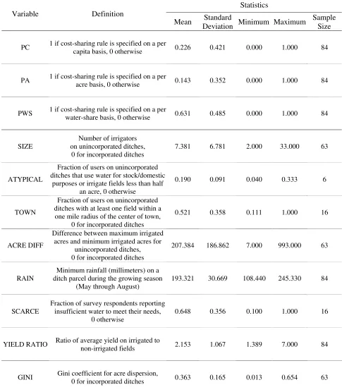
Table 1 reports the definitions of the variables and various summary statistics. Notice that
the sample is unbalanced in the direction of per water-share rules, with the precise distribution
being per water-share (n = 53), per capita (n = 19) and per acre (n = 12) rules. Due to the
manner in which the data are recorded, we do not have information on SIZE, TOWN, ACRE
DIFF and GINI for the 21 incorporated ditches. For the 63 unincorporated ditches, there is an
average of approximately seven users with most users living outside town. There is also
substantial variation in irrigated acres, either measured by ACRE DIFF with a mean of 207 or by
GINI with a mean of 0.363. The ATYPICAL variable indicates that most ditches are comprised
of larger users who are irrigating crops – only six ditches have users who are irrigating small
acreage or are using the water for stock or domestic purposes. There is substantial variation in
RAIN (with the minimum rainfall varying between 108 and 245 millimeters per growing season)
and in YIELD RATIO (with a minimum of 1.4 and a maximum of 7.0). Finally, SCARCE
indicates that for 43 of the 59 reporting ditches, all of the corresponding survey responses assert
that there is sufficient water to meet all irrigation needs. Of the remaining 16 ditches, an average
of two-thirds of the respondents report limited water availability.
4. Econometric Analysis
In this section, we introduce the econometric models and the estimation methods. The
11
can explain the actual choice of equity bases and whether this explanatory power is consistent
with benefit inequity, and other axiomatic principles.
We consider two different estimation frameworks. In the first, we treat the choice of equity
basis as a two-stage binary decision estimated with sequential probit models. In stage one, the
agents choose whether the equity basis should be per capita or selected amongst the remaining
two alternatives. If not, then in stage two the agents choose between per acre and per
water-share equity bases. An advantage of this approach over the traditional multinomial logit model is
that it allows for a more parsimonious model in stage one. Because per capita allocations are
transparent and easy to calculate, agents may naturally gravitate toward the per capita basis
unless there is sufficient variation in benefits to cause them to consider other bases. Consistent
with this “go simple unless there is a compelling reason to the contrary – axiom,” we assume that
agents use a small set of simple structural indicators to determine if the per capita basis is an
equitable choice. Once this initial choice is determined, ditches that did not select the per capita
basis use a larger and more sophisticated set of structural indicators to narrow the choice
between the per acre and per water-share variants.
A disadvantage of the two-stage approach is that it restricts decisions to be made
sequentially, such that the second-stage decision between per acre and per water-share bases is
made without consideration of the per capita basis. With the multinomial logit model, we relax
this assumption by allowing agents to consider all three equity bases simultaneously using the
full set of structural factors. However, because the multinomial logit model effectively imposes
the “independence of irrelevant alternatives” (IIA) assumption, we perform a Hausman test to
see if agents do indeed decide between per acre and per water-share bases independent of the per
12
4.1Bivariate Probit
We begin by assigning the irrigation ditch as the unit of observation, which is indexed from
i = 1,…,n. In our first model, we restrict irrigators to select a per capita basis or to select from
the set of all other alternatives. This choice of equity basis is in turn assumed to depend on
structural characteristics as indicated by the following equation:
PCi*= Xi′β +εi , (2)
where PCi*is a latent variable measuring the likelihood of choosing the per capita basis for ditch
i, Xi is a column vector of explanatory variables for ditch i thought to influence the choice of
equity basis, β is a column vector of coefficients, and εi is a normally distributed error term with
mean zero. By assuming a normal distribution, we then form the likelihood function conditional
on the observed data. Letting F denote the cumulative density function associated with the error
term, we can write the probability that the ith ditch chooses the per capita equity basis (indicated
by PCi = 1) as:
Pi=Pr(PCi = 1) = Pr(PCi* > 0) = Pr(εi > – Xi′β ) = F(Xi′β ). (3)
The probability that the ith ditch adopts either the per acre or per water share basis (PCi = 0) is
therefore given by 1 – Pi = F(Xi′β ). Assuming independence of error terms, we can then write
13 ln(L)= i=1[PCi
n
∑
ln(Pi)+(1−PCi)ln(1−Pi)]. (4)The problem of forming and maximizing (4) by choosing β, given normally distributed error
terms, is referred to as the probit model. This estimation procedure requires nonlinear
optimization techniques to generate estimates of the β parameters and the associated marginal
effects (Greene, 2008).5
In stage two, ditches that did not select the per capita equity basis, then decide between per
acre and per water-share bases. This model is given by
PAj*=Zj′γ + νj, (4)
where j indexes all ditches that did not choose the per capita equity basis in stage one, PAj* is a
latent variable measuring the likelihood of choosing the per acre equity basis, Zj is a column
vector of explanatory variables for ditch j thought to influence the choice of equity basis, γis a
column vector of coefficients, and νj is a mean-zero, normally distributed error term. The log
likelihood function is then formed and maximized to obtain estimates of γand the associated
marginal effects.
4.2Multinomial Logit
We also consider a model where agents on each ditch choose simultaneously from amongst
the per capita, per acre, and per water share equity bases. The model can be written as
5 The estimation was carried out in Gauss 8.0 using the Constrained Maximum Likelihood (CML) module and
14
PCi*=Zi′β1 + ε1,i (5.1)
PAi*= Zi′β2 + ε2,i (5.2)
where the disturbances ε1,i and ε2,i are assumed to be independent and follow a type 1 extreme
value distribution (Greene, 2008). This leads to the following probabilities
P1,i = Pr(PCi = 1) = exp(Zi′β1)/(1 + exp(Zi′β1) + exp(Zi′β2) (6.1)
P2,i = Pr(PAi = 1) = exp(Zi′β2)/(1 + exp(Zi′β2) + exp(Zi′β2) (6.2)
P3,i = Pr(PWSi = 1) = 1 – P1,i – P2,i (6.3)
and log likelihood function
ln(L)= i= ⎡⎣PCiln(P1,i)+PAiln(P2,i)+PWSiln(P3,i)⎤⎦
1
n
∑
. (7)Because the multinomial logit model assumes independent and homoscedastic error terms, it
implies that the log-odds ratio between any two choices does not depend on the third choice. As
mentioned above, we test the IIA assumption using a Hausman test.
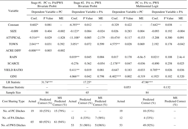
4.3Discussion of the Results
The estimation results are presented in Table 2. Let us begin with the stage-one estimation
results using all 84 ditches. We consider four explanatory variables: SIZE, ATYPICAL, TOWN
15
greater differences in the benefits realized by irrigators on the ditch and thus the benefit inequity
principle would suggest there is pressure to adopt an equity basis other than per capita. The
effect of TOWN is not as clear, although we expect that users near town will tend to be more
uniform in the benefits received from ditch access. Our priors are supported by the econometric
results – large rural ditches with atypical users and greater variation in irrigated acres are less
likely to choose the per capita equity basis. The coefficients of ATYPICAL, TOWN, and ACRE
DIFF are all statistically significant at the 5% level. In terms of goodness-of-fit, the likelihood
ratio test indicates that the model explains a significant amount of the variation in the use of the
per capita equity basis. The model correctly predicts 70 of the 84 ditches while a maximum
score (MS) estimator, a semi-parametric estimator that directly maximizes the number of correct
predictions, predicts 76 of the 84 ditches.6
In stage two, the 65 remaining ditches choose between per acre and per water-share bases.
Agents on the ditch consider a larger and more sophisticated set of explanatory variables in
deciding between these two bases than they did in stage one. In addition to the explanatory
variables from stage one, we consider RAIN, SCARCE, YIELD RATIO and GINI. GINI is a
more sophisticated measure of the variation in irrigated acres than ACRE DIFF. To avoid
multicollinearity issues, we exclude ACRE DIFF from stage two.
We expect that higher values for SIZE and ATYPICAL are likely to be associated with
greater variation in the use and quality of the land, both of which suggest greater variation in the
benefits received from irrigating a given acre. As such, the benefit inequity principle would tend
to decrease the chance that a per acre basis is chosen. Conversely, we expect that land clustered
6 The coefficient estimates for the MS estimator have the same sign as those from the probit model and are available
16
near a town will be more uniform in both its quality and use, which in turn leads to a greater
likelihood of the per acre basis. Therefore, the coefficient on TOWN is expected to be positive.
RAIN, SCARCE, and YIELD RATIO do not speak directly to variation in the quality of
land, but do speak (each in a different way) to the variation in benefits realized by a given
distribution in land quality. Ample rainfall tends to lessen the incremental per acre benefits of
irrigation, thus reducing the variation in acre benefit and making the per acre basis more likely.
Greater water scarcity suggests that the benefits of receiving the water are larger, benefit
variation is amplified, and the per acre basis is less likely to be selected. A higher YIELD
RATIO tends to indicate lower quality land and thus for a given amount of rain and availability
of irrigation water there will be less benefit variation from irrigation on a per acre basis. As
such, we expect higher values of YIELD RATIO to lead to a greater likelihood of per acre basis
adoption. Finally, values of GINI do not directly speak to variation in the benefits received on
individual acres. However, larger values of GINI tend to indicate that variation in benefits can
be more fully explained by just the variation in the number of acres, suggesting that a per acre
basis is more likely to be adopted. All the coefficient estimates are statistically significant except
for SCARCE and have signs consistent with the discussion above. The probit model correctly
predicts 55 of the 65 ditches while the MS estimator correctly predicts 59 ditches.
Finally, we discuss the estimation results from the multinomial logit model. The multinomial
logit model allows the simultaneous selection from amongst the alternative equity bases while
considering the full set of explanatory variables. Overall, the model has significant explanatory
power (likelihood ratio statistic is 47.96, significant at the 1% level) and is able to correctly
predict 75% (63 of the 84) of the equity bases. We highlight several salient features from the
17
First, the most significant determinants of the per capita basis are TOWN, SCARCE and
GINI. The marginal effects indicate, all else equal, that an increase in the fraction of users
residing in town from 0.25 to 0.75 will increase the probability of choosing the per capita basis
by 0.035 percentage points. Likewise, a decrease in GINI or SCARCE from 0.5 to 0.25
increases the probability of choosing the per capita basis by 0.08 and 0.02 percentage points,
respectively. All the coefficients in the PC equation have the expected sign – large ditches in
town with more rain have an increased chance of using the per capita basis; while ditches with
atypical users, increased water scarcity, and greater variation in irrigated acres are less likely to
employ the per capita basis.
Second, the two most significant factors that lead to the choice of a per acre basis are the
yield ratio and the variation in irrigated acres. For example, if the ratio of yield from irrigated to
non-irrigated land doubled from 1 to 2, the probability of choosing the per acre basis would
increase by 0.036 percentage points, all else equal. An increase in the Gini index from 0.25 to
0.5 leads to an increase in the probability of choosing the per acre basis by 0.08 percentage
points, all else equal. The coefficient on RAIN is positive as expected and significant at a 15%
level.
Third, although the magnitude of the coefficients between the probit and multinomial logit
models differs, they are qualitatively similar. This provides a degree of confidence that the
two-stage approach and the IIA assumption of the multinomial logit are reasonable. Furthermore, the
Hausman statistic to test the IIA assumption in the PA equation of the multinomial logit is 0.132
with chi-squared (df = 7) critical value equal to 14.1. Therefore, we fail to reject the IIA
hypothesis and the choice between per acre and per water-share bases can apparently be made
18
The empirical results represent a robust relationship between environmental parameters and
the observed equity basis selection. We experimented with several alternative explanatory
variables and various definitions of the current explanatory variables. For instance, we examined
measures of the slope, roughness, and elevation of the land; ditch length; alternative threshold
values for ATYPICAL and TOWN; alternative measures of acre variation such as standard
deviation and normalized ACRE DIFF; rainfall and yield variation; imputation of missing SIZE
observations; and self-reported variation in water usage, to name a few. The coefficients from
these various specifications exhibited the expected signs and the models explained a significant
amount of the variation in the dependent variables. In sum, the empirical analysis appears to
indicate a robust and stable relationship between features of the allocation environment and the
chosen equity basis.
5. Conclusion
Cooperative environments are frequently endowed with multiple bases for assessing the
“fairness” of a proposed allocation. Rather than simply take this equity basis selection as given,
we have sought to determine whether parameters of the cooperative environment could be used
to effectively explain this selection. Moreover we have sought to establish whether this
explanatory power, to the extent that it existed, was consistent with axiomatic principles of
collective behavior. Our results have confirmed that both of these questions can be answered
affirmatively. Using irrigation sharing data, we have demonstrated that features of the
cost-sharing environment enjoy substantial explanatory power in determining the equity basis
embraced in practice. This explanatory power is consistent with the benefit inequity principle –
19
selection. As such, our empirical results are also supportive of an axiomatic approach to cost
allocation applications.
In closing, we note that an important first step in the forging of stable and mutually beneficial
cooperative agreements is the selection of an appropriate basis for equity assessment. Our
analysis can be viewed as providing guidance on the best way to select such a basis. Indeed, the
understanding of how environmental features can be used to explain the foundations for
successful, well-established cooperative ventures can in turn be used to help construct the
20
6. References
Aadland, D. and V. Kolpin, 2004. Environmental determinants of cost sharing. Journal of Economic Behavior and Organization, 53, 495-511.
Ashton J. and X. Wang, 2003. Equity and climate: in principle and practice. In: Beyond Koyoto: advancing the international effort against climate change. Pew Center on Global
Climate Change, 61-84.
Cohen, J. and P. Cohen, 1983. Applied multiple regression/correlation analysis in behavioral sciences. 2nd ed., Erlbaum, Hillsdale, NJ.
Greene, W. H., 2008. Econometric Analysis. 6th ed., Prentice Hall, Upper Saddle River, NJ.
Grossman, J., 2001. Blue planet: the Kyoto fairness issue. UPI Science News. United Press International.
Hausman, J. and D. McFadden, 1984. Specification tests for the multinomial logit model.
Econometrica, 52, 1219-40.
Lambert, P, 2002. The Distribution and Redistribution of Income. 3rd ed. Manchester University Press, Manchester, UK.
Littlechild, S. C. and G. Owen, 1973. A simple expression for the Shapley value in a special case. Management Science, 20, 370-2.
Nash, J. F., 1950. The bargaining problem. Econometrica, 28, 155-62.
Oregon Climate Service, 2002. http://www.ocs.orst.edu.
Sen, A., 1973. On Economic Inequality. Clarendon Press, Oxford, UK.
Shapley, L. S., 1953. A value for n-person games. In: Contributions to the Theory of Games, vol II, H. W. Kuhn and A. W. Tucker, eds. Annals of Mathematics Studies 28. Princeton University Press, Princeton, NJ, pp. 307-17.
USDA Soil Conservation Service and Forest Service, 1975. Soil Survey of Carbon County Area, Montana.
USDA Soil Conservation Service, 1980. Soil Survey of Stillwater County Area, Montana.
Water Resource Division of the Montana DNRC, 2002.
21
Table 1. Variable Definitions and Descriptive Statistics
Statistics Variable Definition
Mean Standard
Deviation Minimum Maximum
Sample Size
PC 1 if cost-sharing rule is specified on a per capita basis, 0 otherwise 0.226 0.421 0.000 1.000 84
PA 1 if cost-sharing rule is specified on a per
acre basis, 0 otherwise 0.143 0.352 0.000 1.000 84
PWS 1 if cost-sharing rule is specified on a per
water-share basis, 0 otherwise 0.631 0.485 0.000 1.000 84
SIZE
Number of irrigators on unincorporated ditches,
0 for incorporated ditches
7.381 6.781 2.000 33.000 63
ATYPICAL
Fraction of users on unincorporated ditches that use water for stock/domestic
purposes or irrigate fields less than half an acre, 0 otherwise
0.190 0.091 0.040 0.333 6
TOWN
Fraction of users on unincorporated ditches with at least one field within a one mile radius of the center of town,
0 for incorporated ditches
0.521 0.358 0.111 1.000 16
ACRE DIFF
Difference between maximum irrigated acres and minimum irrigated acres for
unincorporated ditches, 0 for incorporated ditches
207.384 186.862 7.000 993.000 63
RAIN
Minimum rainfall (millimeters) on a ditch parcel during the growing season
(May through August)
193.321 30.669 108.440 245.330 84
SCARCE
Fraction of survey respondents reporting insufficient water to meet their needs,
0 otherwise
0.648 0.356 0.100 1.000 16
YIELD RATIO Ratio of average yield on irrigated to non-irrigated fields 2.153 1.067 1.389 7.000 84
GINI Gini coefficient for acre dispersion, 0 for incorporated ditches 0.363 0.165 0.013 0.654 63
22
Table 2. Estimation Results: Choice of Equity Basis for Irrigation Cost-Sharing Rules Stage #1. PC vs. PA/PWS
Bivariate Probit
Stage #2. PA vs. PWS Bivariate Probit
PC vs. PA vs. PWS Multinomial Logit
Dependent Variable = PC Dependent Variable = PA Dependent Variable = PC Dependent Variable = PA Variable
Coef. P Value ME Coef. P Value ME Coef. P Value ME Coef. P Value ME
Constant 0.602* 0.081 -- -6.393** 0.012 -- -0.329 0.422 -- -7.642** 0.038 --
SIZE -0.009 0.404 -0.002 -0.123* 0.084 -0.024 0.026 0.283 0.004 -0.093 0.192 -0.004
ATYPICAL -9.514** 0.029 -1.828 -11.108* 0.085 -2.179 -10.474† 0.117 -0.153 -5.208 0.300 0.091
TOWN 2.041** 0.031 0.392 3.051* 0.072 0.599 4.575** 0.028 0.069 2.192 0.178 -0.042
ACRE DIFF -0.008*** 0.003 -0.002
RAIN 0.019** 0.045 0.004 0.017 0.170 -6.0e-5 0.021† 0.108 2.4e-4
SCARCE -0.276 0.362 -0.054 -2.178** 0.047 -0.036 -0.890 0.258 0.025
YIELD RATIO 0.411** 0.019 0.081 -0.647 0.183 -0.033 0.705** 0.026 0.036
GINI 4.066** 0.042 0.798 -8.402*** 0.002 -0.319 4.192† 0.102 0.320
LR Statistic 31.74*** 17.25* 47.96***
Hausman Statistic -- -- 0.053 0.132
Sample Size 84 65 84
Cost Sharing Type Actual Predicted Correct (%) MS Predicted Correct (%) Actual Predicted Correct (%) MS Predicted Correct (%)
Actual Predicted
Correct (%)
MS Predicted Correct
(%)
No. of PC Ditches 19 10 (53%) 15 (79%) -- -- -- 19 10 (53%) --
No. of PA Ditches 12 4 (33%) 7 (58%) 12 4 (33%) --
No. of PWS Ditches
65 60 (92%) 61 (94%)
53 51 (96%) 51(96%) 53 49 (92%) --