Alternative Tilts for Nonparametric
Option Pricing
Walker, Todd B and Haley, M. Ryan
Indiana University
6 September 2009
M. Ryan Haley
∗Todd B. Walker
†13 July 2009
Abstract
This paper generalizes the nonparametric approach to option pricing of
Stutzer(1996) by demonstrating that the canonical valuation methodology in-troduced therein is one member of the Cressie-Read family of divergence mea-sures. While the limiting distribution of the alternative measures is identical to the canonical measure, the finite sample properties are quite different. We assess the ability of the alternative divergence measures to price European call options by approximating the risk-neutral, equivalent martingale measure from an empirical distribution of the underlying asset. A simulation study of the finite sample properties of the alternative measure changes reveals that the optimal divergence measure depends upon how accurately the empirical distri-bution of the underlying asset is estimated. In a simple Black-Scholes model, the optimal measure change is contingent upon the number of outliers observed, whereas the optimal measure change is a function of time to expiration in the
stochastic volatility model of Heston (1993). Our extension of Stutzer’s
tech-nique preserves the clean analytic structure of imposing moment restrictions to price options, yet demonstrates that the nonparametric approach is even more general in pricing options than originally believed.
Keywords: Option Pricing, Nonparametric, Entropy
JEL Classification Numbers: G13, C14
1
Introduction
Due to the poor empirical performance of parametric models, nonparametric option pricing techniques have expanded rapidly in recent years [Hutchinson, Lo, and Poggio (1994), Rubenstein (1994), A¨ıt-Sahalia and Lo (1998), (Broadie, Detemple, Ghysels, and Torres, 2000), Garcia and Gen¸cay (2000)]. Duan (2002) lays out two important criticisms of these nonparametric methods. First, many of these techniques, such as neural networks and kernel regressions, suffer from the curse of dimensionality; i.e., they require large amounts of option pricing data to perform well. Second, many of these techniques are unable to price options of different maturities and therefore do not exploit all of the available cross-sectional information [e.g., Buchen and Kelly (1996)]. This weakness arises because the nonparametric risk-neutral distributions are identified separately according to contract maturity. Therefore, neither the statistical properties of the underlying asset nor the properties of the option prices at different maturities can be used to price options of a specific maturity. This also implies that these techniques cannot be used to price path-dependent derivatives (e.g., barrier options). When pricing redundant securities (as is our focus here), these shortcomings are potentially severe.
In contrast, the nonparametric method of Stutzer (1996) (referred to as canonical valuation) does not require any option pricing data and takes full advantage of the available cross-sectional information. The defining feature of Stutzer’s approach is the maximum cross-entropy (or minimum Kullback-Leibler) technique, which minimizes the divergence between the actual probability distribution governing the underlying asset and its risk-neutral counterpart needed to price the derivative security. This minimization is subject to the constraint that the underlying asset price follow a martingale, thus ensuring that the risk-neutral density is in fact of the correct form. Cross-sectional information is imbedded into the estimation process through moment restrictions by imposing that the risk-neutral density correctly price options of the same maturity by different strikes.
dramatically when pricing options in a stochastic volatility world.
The goal of this paper is to test alternatives to the canonical valuation ofStutzer (1996) by generalizing the problem of finding a minimum divergence between the ac-tual and risk-neutral distribution. This generalization is possible because the cross-entropy between two distributions is a special case of the Cressie-Read divergence family. We examine how well other members of the Cressie-Read family (e.g., Eu-clidean divergence and empirical likelihood divergence) price a European call option in a simulated Black-Scholes environment and stochastic volatility environment. We find that in certain situations, the alternative measure changes outperform the canon-ical estimator. More specifcanon-ically, in the Black-Scholes environment we find that the number of outliers observed plays a crucial role in determining the accuracy of the nonparametric method. For reasons described below, the empirical likelihood es-timator does a better job of handling outliers and thus outperforms the canonical estimator. This result is robust to different maturities and across several different types of moneyness. This result is also robust to different types of pricing errors (mean-percentage and mean-absolute pricing errors).
In the stochastic volatility simulation, we show that the optimal measure change depends critically on the time to expiration; this result is robust to different levels of moneyness but is not robust across the different types of pricing errors. Mean pricing errors are dramatically reduced by generalizing the option pricing method. Absolute pricing errors, however, are only significantly different for specific maturity structures and moneyness. Moreover, we simulate from the stochastic volatility model using the method of Broadie and Kaya(2006), which drastically reduces the discretization bias hence making it possible to distinguish between discretization error and pricing error. This paper also contributes to the applied econometrics literature by examin-ing the finite sample properties of various nonparametric estimation methods. Non-parametric methods, such as empirical likelihood, have become increasingly popular among economists and statisticians [Kitamura (2005)] but relatively little is known about the finite sample properties of these alternative estimators.1 The pricing of
op-tions is an ideal environment to study these finite sample properties because changes of measure (from actual to risk-neutral probabilities) are fundamental to pricing deriva-tive securities and therefore, the properties of these measure changes are well known. While we are not performing “full-blown” estimation (i.e., optimizing over a param-eter set) as is typically done in econometric applications, we are able to accurately assess how alternative measure changes behave in small samples.
1
2
Nonparametric Pricing of Options
Consider pricing a European call option with expiration date T and strike price X. In the absence of arbitrage, the price of the European call optionC discounted at the risk-free rate of interest r is given by
C =EQt
max[PT −X,0]
(1 +r)T
, (2.1)
where PT is the price of the underlying asset at date T, and EQt implies that the
expectation is taken with respect to the risk-neutral (equivalent-martingale) measure. Suppose one had on hand a time series of underlying stock prices, denoted by pt, of
lengtht = 1, ..., T−h, wherehis the number of days to expiration. In lieu of imposing a specific functional form on the price process of the underlying asset,Stutzer (1996) advocates forming the empirical distribution of time T asset returns (assuming the stock does not pay a dividend) by forming
Rt =
pt+h
pt
t= 1, ..., N (2.2)
and weighting each draw equally, πt=N−1 for all t, where N =T −2h.2
Of course, the weights associated with the empirical distribution (πt = N−1)
are not the risk-neutral weights needed to price the option (2.1). Thus, we seek a transformation from the “real-world” probabilitiesπtto their risk-neutral counterpart
πtQ, where the risk-neutral weights satisfy
N
X
t=1
πtQ = 1, (2.3)
1 =
N
X
t=1 πtQ
Rt
(1 +r)T
. (2.4)
Equation (2.3) requires the risk-neutral weights sum to one, and more importantly, (2.4) forces the risk-neutral weights to satisfy the martingale property. Risk-neutral weights that satisfy the above restrictions can then be used to price the option ac-cording to
C =EQt
max[PT −X,0]
(1 +r)T
=
N
X
t=1 πQt
max[PT −X,0]
(1 +r)T
(2.5)
Therefore, we seek a change of measure from π = [π1, ..., πN]′ to πQ = [π1Q, ..., π
Q N]′
that satisfies (2.3) and (2.4) but does not diverge too far (as per some measure-change metric) from the underlying asset’s empirical distribution.
2
2.1
Canonical Valuation
Stutzer (1996) controls the divergence between the two measures by minimizing their cross-entropy or Kullback-Leibler divergence. Define the cross-entropy as
CE(πtQ, πt) = N
X
t=1
πtQlog
πtQ πt
. (2.6)
Minimizing (2.6) subject to (2.3) and (2.4) is a well-defined convex minimization problem. Stutzer refers to this nonparmetric option pricing technique as canonical valuation (CAN) because the solution takes the form of the Gibbs canonical distri-bution
πQt,CAN = exp γ
QR
t(1 +r)−T
PN
t=1exp γQRt(1 +r)−T
whereγQis the Lagrange multiplier satisfying,γQ = arg min
γPNt=1exp
γ Rt (1+r)T−1
.
As mentioned in the introduction, this approach can also easily incorporate cross-sectional option pricing data, if it is available. For example, incorporating an option that matures at the same date but has a different strike X2 and option price C2 can be achieved by simply adding the constraint
C2 =
N
X
t=1 πtQ
max[PT −X2,0]
(1 +r)T
(2.7)
to (2.4) and (2.3), and minimizing (2.6).
Given the nice theoretical structure of the problem, it is computationally inexpen-sive to price options employing this method; simple Excel computations are sufficient. Moreover, the CAN estimator has been shown to accurately (vis-a-vis alternative op-tion pricing methods) price opop-tions in realistic settings [Gray and Newman (2005)].
2.2
Alternative Measure Changes
The CAN estimator is one method for deriving the risk-neutral distribution from an estimate of the actual distribution. However, the problem of finding an equivalent martingale measure may be generalized by defining a convex function Ψ that measures the divergence between two probability measuresP (actual probabilities) andQ (risk-neutral probabilities):
D(Q, P) =
Given an appropriate choice of Ψ, we seek minimization of (2.8) subject to the con-straints (2.3) and (2.4).3
Specifically, we examine the Cressie-Read (CR) divergence family as a choice for the convex function Ψ(x) [Cressie and Read (1984), Baggerly (1998)]. The CR divergence between the actual and risk-neutral probability measure is defined by
CRλ(πtQ, πt) =
2
λ(1 +λ)
N
X
t=1 πt
πQt
πt
−λ
−1
,
for a fixed scalar parameter λ.
The choice of the CR divergence stems from the fact that it generalizes several well-known divergence measures, including the cross-entropy measure. For example,
λ = −2 yields the Euclidean divergence, λ = 1 gives Pearson’s Chi-Square, and
λ =−1/2 is the squared Hellinger divergence. Two limiting distributions which are also encountered frequently are empirical likelihood (λ → 0) and the cross-entropy measure (λ→ −1) (see, Bera and Bilias(2002) for a nice review).
Our motivation behind examining alternative measure changes can be clearly seen by factoring the CR objective function according to Basu and Lindsay(1994);4
CRλ(πtQ, πt) =
2
λ(λ+ 1)
N X t=1 πt πt
πtQ
λ
−1
+λ(πtQ−πt)
= 2
N
X
t=1
D(δt, λ)πQt (2.9)
where
D(δ, λ) = (δ+ 1)
λ+1−(δ+ 1) λ(λ+ 1) −
δ
λ+ 1, δt=
πt
πQt −1
.
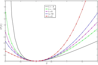
Thus, the CR divergence may be interpreted as a weighted function (D) of disparity measures (δ) between the actual and risk-neutral probability measures. The function
D(·) is non-negative, defined on [−1,∞) and equals zero if and only if the disparity between the two measures is also zero. Figure 1 plots this disparity measure for
λ= [−2,−0.5,0,2,0.5].5
Note that for positive (negative) values of δ, positive (negative) λ lead to higher values for D. Thus CR divergence measures with positive (negative) λ restrict the
3
This type of estimation is often referred to as Generalized Minimum Contrast (GMC). The obvious benefit of GMC estimation is the lack of distributional assumption. Moreover, the GMC estimator is shown to possess properties similar to that of parametric likelihood estimators [Kitamura and Stutzer(1997),Kitamura(2005)].
4
Note that the termλ(πQt −πt) does not contribute to the disparity.
5
[image:7.612.130.523.366.517.2]degree to which the actual (risk-neutral) probability can exceed the risk-neutral (ac-tual) probability. For the option pricing problem at hand, this implies that if the empirical distribution has fatter tails than the actual distribution, then CR measures with negative lambda will, on average, be more accurate in pricing the option. Con-versely, if the empirical distribution has thinner tails than the actual distribution, then CR measures with positive lambda will be more accurate in pricing the option. This is precisely how finite samples lead to different performance metrics for different CR measures.
An alternative, and perhaps more powerful, motivating factor for our approach is to consider the risk appetite of the investor. Haley, McGee, and Walker (2009) show that the alternative tilts of the CR metric correspond to different HARA utility functions. The implication for option pricing is that if the investor is concerned with minimizing tail risk, then selecting a CR measure with a positive lambda will mitigate pricing errors. Conversely, if the investor believes the market will be less volatile over the life of the option, then a negative lambda will more accurately price the option.
Within the context of option pricing, this interpretation speaks specifically to the persistent negative bias of the CAN estimator documented by Gray and Newman (2005). Our interpretation of this negative bias is that the CAN estimator (λ → −1) is not symmetric about zero and therefore it weights outliers and inliers non-uniformly (down-weighting outliers disproportionately). In order for the CAN estimator to ac-curately price the option, the empirical distribution must have fatter tails (significant number of outliers) relative to the the actual distribution. The simulation results reported below average over thousands of repetitions, and document the persistent negative bias in the CAN estimator. Conversely, note that λ → 0 is more symmet-ric about zero than CR divergence measures with negative λ, implying a more equal weight is given to both inliers and outliers. This suggests that as the number of draws from the empirical distribution increases (and assuming one is able to sample from the entire support of the distribution), the empirical likelihood (λ → 0) divergence measure should lead to the smaller mean pricing errors due to its more symmetric divergence shape. The upshot is that if the empirical distribution is not representa-tive of the actual distribution needed toforecast future values of the underlying asset, then depending upon the bias, alternative CR divergence measures will outperform the CAN estimator.
This paper will focus on three members of the CR family–the canonical estimator (λ→ −1), the empirical likelihood estimator (λ →0), and the Euclidean divergence (λ=−2). There are two motivating factors for the selection of these three estimators. First, these estimators have recently been advocated in various econometric settings and the properties of these estimators are becoming well known.6 Second, the
compu-6
This literature has become too voluminous to accurately cite all the works that should be given credit. Imbens, Spady, and Johnson (1998), Hansen, Heaton, and Yaron (1996), Kitamura and Stutzer (1997), andNewey and Smith (2004) are among the important recent contributions. Both
−1 −0.5 0 0.5 1 1.5 2 0
0.2 0.4 0.6 0.8 1 1.2 1.4 1.6 1.8 2
λ = − 2 λ = − 1/2 λ = 0 λ= 1/2 λ = 2
D
(
δ
)
[image:9.612.99.499.90.357.2]δ
Figure 1: Disparity measures for various λ
tational cost to calculate these three estimators is minimal. In the financial industry, where millions of repetitions like those performed below are executed daily, it is im-portant to keep relative computational cost low. Stutzer(1996) demonstrates the ease of computation associated with the the canonical estimator. The total computational time in calculating the Euclidean divergence and empirical likelihood estimators is even less than the canonical estimator.
The formal derivation for these estimators can be found by forming the Lagrangian that minimizes the CR divergence and solves (2.1) subject to (2.3), (2.4) and (2.7). This is given by
L(πQ, k1,k2) =
2
λN(λ+ 1)
N
X
t=1
{(NπQt )−λ−1}+k
1(1−
N
X
t=1
πtQ) +k2′
η−
N
X
t=1 πtQft
where ft= [Rt/(1 +r)T,max{PJ−X,0}/(1 +r)T]′ and η= [1, C2]. Setting ∂L/∂πtQ
to zero yields extremum of the form
πtQ =
(
1
N{1 +c1+c2′(ft−η)}−
1/(λ+1) λ 6=−1 c1exp{c2′(f
t−η)} λ =−1
1)/h= log(t), one can also show
lim
λ→0CRλ(π
Q
t , N−1) =−2 log(πtQN), lim
λ→−1CRλ(π
Q
t , N−1) = 2πtQlog(NπQt )
which is minus twice the empirical log likelihood, and twice the cross-entropy. This shows the close relationship between empirical likelihood and cross-entropy and also makes clear why the empirical likelihood treats outliers uniformly while the canonical estimator does not.
The following proposition derives the risk-neutral weights associated with the empirical likelihood and Euclidean estimators.
Proposition 2.1. The equivalent-martingale measures for the empirical likelihood
and Euclidean estimators that price (2.1) subject to (2.3), (2.4) and (2.7) are given by
πtQ,EL =
1
N
1 1 +k′
2(ft−η)
(2.10)
πtQ,EU = 1
N[1 +k
′
2(ft−¯ft)] (2.11)
Proof. Employing Lagrange multipliers, the constrained optimization problem for minimizing the empirical likelihood is
LEL=−
1
N
N
X
t=1
log(πQt N) +k1(1−
N
X
t=1
πtQ) +k2′
η−
N
X
t=1 πtQft
The first-order conditions are
LπtQ : −
1
πtQN +k1+k
′
2ft = 0 → πtQk1+πtQk′2ft=
1
N (2.12)
Lk2 : η− N
X
t=1
πtQft= 0
Lk1 : 1−
N
X
t=1
πtQ = 0
Summing (2.12) over the N periods gives, k1PN
t=1π
Q t +k′2
PT
t=1π
Q
t ft = 1, and the
other first-order conditions imply k1 = 2−k′
2η. Concentrating out k1 from (2.12)
gives
πtQ = 1
N
1 1 +k′
2(ft−η)
Settingλ=−2 corresponds to the Euclidean divergence, also known as Neyman’s
χ2. Form the Lagrangian according to
LEU =
1 2N
N
X
t=1
(πtQN −1)2+k1(1− N
X
t=1
πtQ) +k2′
η−
N
X
t=1 πtQft
LπtQ : Nπ
Q
t −1 +k1−k′2ft= 0→ k1 = 1 +k′2ft−NπtQ
Averaging over t gives, k1 =k′
2¯ft, and therefore
πtQ = 1
N[1 +k
′
2(ft−¯ft)]
The numerical speed and precision of these estimators comes from the nice func-tional forms of the Lagrangian multipliers. For example, Owen (2001) shows the multiplier for the Euclidean estimator simplifies to k2 =S−1(¯f
t−η) where
S =N−1PN
t=1(ft−¯ft)(ft−¯ft)′.
3
Assessing Alternative Tilts
This section assesses the fit of alternative measures of divergence numerically by assuming the stock process follows specific functional forms that allow for analytical solutions to the option pricing equation (2.1). With analytical solutions in hand, one may examine the pricing errors over a wide range of maturity and moneyness. Pricing errors are calculated followingStutzer (1996) in a Black-Scholes environment. We also followGray and Newman (2005) and examine the pricing errors in the more realist stochastic volatility model ofHeston (1993).
3.1
Alternative Tilts in a Black-Scholes Environment
Both Stutzer and Gray and Newman compare the CAN estimator with implied-volatility estimators by assuming the underlying stock price follows geometric Brow-nian motion
dSt =µStdt+σStdzt,
which gives stock returns as
ln(Rt)∼N[(µ−σ2/2)T, σ2T]. (3.1)
We assign the same parameter values as Stutzer and Gray and Newman; the drift
riskless rate of interest 5%. For each time to expirationT, 200 returns are drawn from (3.1) and the empirical “predictive” distribution for PT is formed according to (2.2).
Also, as a basis for comparison, a Black Scholes implied volatility (HBS) estimate is calculated using the sample volatility in the usual manner. Mean percentage (MPE) and mean absolute percentage (MAPE) pricing errors are then calculated based upon 5,000 repetitions of the experiment.
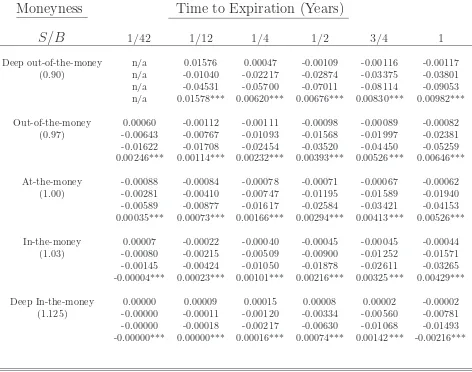
Table 1 reports the MPE results when only one moment restriction (2.4) is em-ployed in the constrained optimization. The table reports results for various time-to-maturities–(assuming 252 trading days) from 6 trading days up to 1 year–and various levels of moneyness–deep out of the money (S/B = 0.9) to deep in the money (S/B = 1.125). The table reports the results listed in order from top to bottom– Black-Scholes, canonical, Euclidean, and empirical likelihood.
Notice that while the HBS estimator consistently prices options across different time to maturities, the nonparametric methods perform worse as the time to expira-tion increases. This is because the HBS estimator needs only to accurately estimate the second moment of the risk-neutral distribution because the parametric assump-tion is correct (that is, the Black-Scholes pricing formula is the correct one here). Conversely, the nonparametric approach re-weights the entire distribution. As the distribution becomes more dispersed, the re-weighting becomes less precise in the nonparametric case, but does not affect the precision of the HBS estimator. The tradeoff is that the HBS estimator makes a dogmatic assumption about the data generating process. If that assumption is correct (as it is here), one only has to match second moments to accurately price options but, as is well documented, the assumption of lognormally distributed returns is empirically implausible.
Second, in almost every case, the EL estimator soundly outperforms the CAN and EU estimators. In many cases, the difference is quite large from an option pricing standpoint and statistically significant. For example, in almost every scenario, the difference in MPE between the EL and the CAN is a factor of 2, and the extreme cases, a factor of 5. Inall cases, paired t-tests reveal the difference between the CAN and EL estimators to be statistically significant at the 99% level. Conversely, the EU estimator performed much worse than the CAN estimator in every scenario with MPEs almost 10 times that of the EL estimators (this difference is also significant at the 99% level). An explanation for this result can be found by examining the number of outliers of the empirical distribution.
0 5 10 15 20 25 −0.15
−0.1 −0.05 0 0.05 0.1 0.15 0.2
EL EU CAN
M
P
E
[image:13.612.124.465.105.350.2]Number of Outliers
Figure 2: Number of Outliers and MPE in Black-Scholes Model Figure 2 plots the average MPE (5,000 simulations) against the number of realizations in 200 draws that were outside of the 2.5th–97.5th percentile range for the given distribution. The average MPE is reported for all moneyness levels and for time to expiration equal to 1/4.
tails than the actual distribution being sampled, then measure changes with positive (negative) lambda will favor larger (smaller) risk-neutral weights relative to negative (positive) lambda measure changes. In other words, alternative measure changes will correct the bias in small samples. This result is important because when applying this nonparametric technique to real-world data, one does not have the luxury of repeated draws from the known distribution. The performance of the nonparametric estimators depends upon the small sample properties of the empirical distribution. As the empirical distribution diverges from the actual distribution, re-weighting the draws may be an important money saving measure. And as table 1 makes clear, these differences can be quite large. This important point can easily be overlooked when conducting Monte Carlo type numerical simulation.
negative delta (πt< πtQ) more heavily, which leads to too low of a price for the option
and hence negative pricing errors.
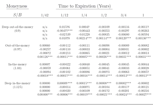
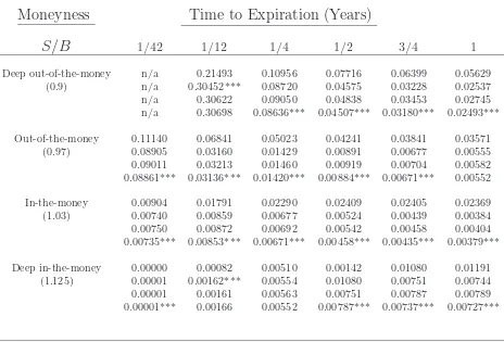
However, the symmetric properties possessed by the EL estimator may not lead to improved performance in pricing options. Table 2 provides the mean absolute pricing errors, which weight negative and positive errors equally. While the superior performance of the EL estimator is again evident, the degree of improvement over the EU and CAN estimators is somewhat tempered when examining the absolute value of the errors–EL outperforms CAN 21 out of the 30 scenarios, a majority of which are statistically significant at the 99% level.
Fourth, Stutzer (1996) argues that in order for the nonparametric method to fairly compared to the HBS estimator an additional moment restriction is necessary. More specifically, imposing that the at-the-money option is correctly priced forces the additional moment restriction
C2 =
N
X
t=1 πtQ
max[PT −X2,0]
(1 +r)T
on the optimization problem. This additional moment restriction is easily incorpo-rated into the problem and doing so alleviates the bias seen in the nonparametric estimators associated with time to expiration. Table 1 documented the increase in MPE for the nonparametric estimators as time to expiration increased. Tables 3 and 4 show that adding the additional constraint effectively eliminates this bias by placing much more structure on the problem. That is, the previous constraint simply imposed the martingale restriction on returns but did not take into account the spe-cific functional form of the asset pricing equation, whereas the HBS estimator always takes into account the particular asset pricing equation. Adding the additional con-straint provides a specific functional form that sufficiently restricts the feasible set of measures such that the corresponding risk-neutral measure is sufficiently close to the actual risk-neutral measure [Stutzer (1996)]. Tables 3 and 4 document that adding the additional constraint dramatically improves the performance of the nonparamet-ric methods. In several instances, the nonparametnonparamet-ric methods outperformed the HBS estimator with the exception of deep in-the-money and deep out-of-the-money calls.
0 50 100 150 200 250 300 350 400 450 500 −0.04
−0.03 −0.02 −0.01 0 0.01 0.02 0.03 0.04 0.05
EL EU CAN HBS
0 50 100 150 200 250 300 350 400 450 500 0.08
0.09 0.1 0.11 0.12 0.13 0.14 0.15 0.16
EL EU CAN HBS
[image:15.612.97.521.92.246.2]3 (a): MPE, T=3/4, S/B=1 3 (b): MAPE, T=1/2, S/B=1.125
Figure 3: Stability of Results. This figure plots the MPE and MAPE for different time-to-expiration and levels of moneyness against the number of simulations.
of simulations increases to 500.
Figure 3(a) plots the MPE for time-to-expiration of 3/4 and moneyness of 1, while 3(b) plots the MAPE for time-to-expiration 1/2 and moneyness 1.125 as the number of simulations are increased to 500.7 As the figure indicates, the ordering
for the estimators occurs quite quickly. After 20 simulations for the MPE and 90 simulations for MAPE, the orderings are established for all estimators. Given that a practitioner would perform these operations over several assets and over a long period of time, the excess profitability of the empirical likelihood estimator vis-a-vis the canonical estimator would be nontrivial. The superior performance of the Black-Scholes estimator and inferior performance of the Euclidean estimator occurs much sooner (roughly 10 simulations). Moreover, this graph is another illustration of the negative bias associated with the canonical estimator (and to a greater extent, the Euclidean estimator), as opposed to the much smaller positive bias in the EL estimator.
3.2
Alternative Tilts in a Stochastic Volatility Environment
Gray and Newman(2005) persuasively argued that a more realistic test of the canon-ical estimator would be to simulate data using Heston’s stochastic volatility model, where the stock price follows
dSt=µStdt+√vtStdz1,t
and the variance of the return follows a Ornstein-Uhlenbeck process
dvt=κ(θ−vt)dt+ξ√vtdz2,t
7
whereκis the speed of mean reversion,θthe long-run variance,ξis the volatility of the volatility generating process, anddz1,t, anddz2,tare Wiener processes with correlation
ρ. The appeal of this setup is that the model retains a closed form solution while providing more realistic simulated data.
To reduce discretization bias in generating the data, we employ the method of Broadie and Kaya(2006).8 The conventional way to generate data from the stochastic
volatility model is to use Euler discretization, but Broadie and Kaya show that this method may introduce substantial bias into the simulated results. They then show how to simulate data from the exact distribution, effectively reducing discretization bias. The data are generated using 1 day time steps and with parameter values given by: stock drift, µ, 10%; long-run mean, θ, 4%; mean reversion, κ, 3; volatility, ξ, 0.4; and correlation, ρ, -0.5. The parameter values follow Gray and Newman, and represent typical estimates from market data.
Tables 5 and 6 give the MPE and MAPE, respectively, for the HBS, CAN, EL, and EU estimators across several maturities and moneyness, assuming 200 draws from the empirical distribution and 5,000 simulations. The obvious disadvantage of the HBS estimator relative to the nonparametric approach is the assumption of an explicit functional form for returns. If the parametric assumption does not fit the data well (as is the case here), the HBS estimator will consistently misprice the option. As indicated in Tables 5 and 6, the HBS estimator overprices out-of-the money options and underprices in-the-money options–a well-known empirical finding. This is primarily due to the fact that the Gaussian distribution, assumed by HBS, has tails that are too thin to adequately capture the dynamics of the SV model. Hence, the HBS estimator is only competitive with the nonparametric estimators if the option has a very short maturity and is at-the-money options.
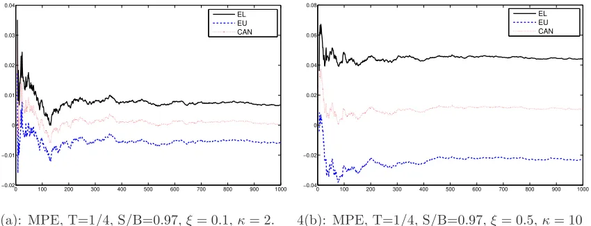
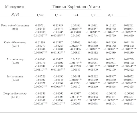
When comparing across the different measure changes in Table 5, an interesting result emerges. Namely, the optimal measure change is a function of the time to expiration. The EL estimator outperforms the other estimators at short time horizons (1/42, 1/12), the CAN estimator outperforms at medium interval (1/4) and the EU estimator outperforms when the time to expiration is greater than 1/2. This result is robust to all levels of moneyness. The intuition for this result is the following; as time to expiration increases, the probability of outliers influencing the returns becomes more likely. The difference here is that the probability of outliers in the SV model is much greater than the Black-Scholes model. Hence the measure change that handles outliers (inliers) the best, EU (EL), will outperform at longer (shorter) horizons. This result is robust to alternative formulations for the stochastic volatility model (not reported) and the differences in pricing errors are statistically significant at the 99% level.9 This result suggests that an optimal portfolio would consist of a
8
We thank Mark Broadie and Ozgur Kaya for permission to use their simulator.
9
0 100 200 300 400 500 600 700 800 900 1000 −0.02
−0.01 0 0.01 0.02 0.03 0.04
EL EU CAN
0 100 200 300 400 500 600 700 800 900 1000 −0.04
−0.02 0 0.02 0.04 0.06 0.08
EL EU CAN
4(a): MPE, T=1/4, S/B=0.97,ξ= 0.1,κ= 2. 4(b): MPE, T=1/4, S/B=0.97,ξ= 0.5,κ= 10
Figure 4: Stability of Results Figure 4 plots the MPE for different parameterizations of the SV model with time-to-expiration of 1/4 and levels of moneyness against the number of simulations.
combination of measure changes contingent upon time to maturity.
However, Table 6 shows that the absolute errors across the alternative measure changes are roughly constant. Unlike the Black-Scholes case, choosing the optimal divergence measure to minimize themean percentage error does not necessarily min-imize the mean absolution percentage errors. Along this dimension, the canonical estimator performed quite well at longer horizons for out-of-the-money and at-the-money options. At shorter maturities, the Euclidean and empirical likelihood esti-mator outperformed. This pattern again suggests a combination strategy that is a function of maturity and moneyness. Many of these differences at the shorter and longer maturities are statistically significant, while at medium maturity there is little difference across the nonparametric estimators.
It should also be noted that adding the additional constraint, (2.7), to the opti-mization dramatically improves the performance of all the nonparametric estimators. Tables 7 and 8 provide the MPE and MAPE when the additional constraint is applied, and indicates, yet again, that the nonparametric method is a viable option pricing strategy. Note also that adding the additional constraint makes the nonparametric estimators nearly identical in performance in terms of absolute pricing errors. This is intuitive because the nonparametric estimators converge as the number of moment restrictions imposed increases. As Table 8 shows, there are still statistically signifi-cant differences across the estimators with respect to shorter maturities, and only for deep-in-the-money calls at longer maturities.
[image:17.612.95.520.92.255.2]estimator dominates the others. This figure is representative of the more general result–the appropriate measure change is a function of time to expiration regardless of moneyness and parameters of the SV model. Moreover, as documented by Figure 4, this result is exacerbated as volatility is increased. That is, the more dispersed the data, the more the optimal measure change will outperform the others. This convergence happens very quickly (less than 50 iterations).
4
Conclusion
In this paper we have examined a generalized version of Stutzer’s (1996) canonical valuation option pricing estimator. We framed our analysis around the Cressie-Read family of divergence measures, which captures Stutzer’s cross-entropy as a special case. Simulations in both Black-Scholes and stochastic volatility environments suggest that the canonical estimator can be significantly improved upon in finite sample scenarios. Of the Cressie-Read divergences we considered, the empirical likelihood divergence demonstrated itself to be an extremely viable alternative to Stutzer’s cross entropy. We trace this advantage back to how each divergence weighs values; we find that the symmetry of the empirical likelihood measure appears to drive its desirable performance. This feature also sheds additional light on the negative bias associated with applications of the canonical estimator as in Gray and Newman (2005). In the stochastic volatility environment, the optimal choice of measure change depended upon the time to expiration. These results suggest that an optimal portfolio approach would advocate for inclusion of all measures of the Cressie-Read divergence family when constructing a nonparametric option portfolio.
References
A¨ıt-Sahalia, Y., and A. Lo (1998): “Nonparametric Estimation of State-Price
Densities Implicit in Financial Asset Prices,” Journal of Finance, 53, 499–547. 1
Alcock, J., and T. Carmichael (2008): “Nonparametric American Option
Pric-ing,”Journal of Futures Markets, 28(8), 717–748. 1, 16
Baggerly, K. (1998): “Empirical likelihood as a goodness-of-fit measure,”
Biometrika, 85(3), 535. 5
Basu, A., and B. Lindsay (1994): “Minimum disparity estimation for
continu-ous models: Efficiency, distributions and robustness,” Annals of the Institute of Statistical Mathematics, 46(4), 683–705. 5
Bera, A.,andY. Bilias(2002): “The MM, ME, ML, EL, EF and GMM approaches
to estimation: a synthesis,” Journal of Econometrics, 107(1-2), 51–86. 5, 6
Broadie, M., J. Detemple, E. Ghysels, and O. Torres (2000): “American
Options with Stochastic Volatility and Stochastic Dividends: A Nonparametric Investigation,” Journal of Econometrics, 94, 53–92. 1
Broadie, M., and O. Kaya¨ (2006): “Exact simulation of stochastic volatility and
other affine jump diffusion processes,” Operations Research, 54(2), 217–231. 2,14
Buchen, P., andM. Kelly(1996): “The Maximum Entropy Distribution of an
As-set Inferred from Option Prices,” Journal of Financial and Quantitative Analysis, 31, 143–159. 1
Cressie, N., and T. Read (1984): “Multinomial Goodness-of-Fit Tests,” Journal
of the Royal Statistical Society. Series B (Methodological), 46(3), 440–464. 2, 5
Duan, J.-C. (2002): “Nonparametric Option Pricing by Transformation,” Working
Paper, Rotman School of Management. 1
Garcia, R., and R. Genc¸ay (2000): “Pricing and hedging derivative securities
with neural networks and a homogeneity hint,”Journal of Econometrics, 94(1-2), 93–115. 1
Gray, P., S. Edwards, andE. Kalotay (2007): “Canonical Pricing and Hedging
of Index Options,”Journal of Futures Markets, Forthcoming. 1,16
Gray, P.,andS. Newman(2005): “Canonical Valuation of Options in the Presence
Haley, M. R., M. K. McGee, and T. B. Walker(2009): “Disparity, Shortfall, and Twice-Endogenous HARA Utility,” mimeo, Indiana University. 6
Hansen, L., J. Heaton, and A. Yaron (1996): “Finite-Sample Properties of
Some Alternative GMM Estimators,” Journal of Business & Economic Statistics, 14(3), 262–280. 6
Heston, S. L.(1993): “A Closed-Form Solution for Options with Stochastic
Volatil-ity with Applications to Bond and Currency Options,”Review of Financial Studies, 6, 327–343. 1, 9
Hutchinson, J., A. Lo, and T. Poggio (1994): “A Nonparametric Approach to
the Pricing and Hedging of Derivative Securities via Learning Networks,” Journal of Finance, 49, 851–889. 1
Imbens, G., R. Spady, and P. Johnson (1998): “Information Theoretic
Ap-proaches to Inference in Moment Condition Models,” Econometrica, 66(2), 333– 357. 6
Kitamura, Y. (2005): “Empirical Likelihood Methods in Econometrics: Theory
and Practice,”Invited paper presented at the Econometric Society World Congress, UCL, London. 2, 5
Kitamura, Y., and M. Stutzer (1997): “An Information-Theoretic Alternative
to Generalized Method of Moments Estimation,”Econometrica, 65(4), 861–874. 5, 6
Maasoumi, E. (1993): “A compendium to information theory in economics and
econometrics,” Econometric Reviews, 12(2), 137–181. 6
Newey, W., and R. Smith(2004): “Higher Order Properties of GMM and
Gener-alized Empirical Likelihood Estimators,”Econometrica, 72(1), 219–255. 6
Owen, A. (2001): Empirical likelihood. CRC Press. 9
Robertson, J. C., E. W. Tallman, and C. H. Whiteman(2005): “Forecasting
Using Relative Entropy,” Journal of Money, Credit, and Banking, 37(3), 383–401. 3
Rubenstein, M. (1994): “Implied Binomial Trees,” Journal of Finance, 49, 771–
818. 1
Stutzer, M. (1996): “A Simple Nonparametric Approach to Derivative Security
Table 1: MPE in Black-Scholes World with 1 Moment Restriction*
Moneyness
Time to Expiration (Years)
S/B
1/42 1/12 1/4 1/2 3/4 1Deep out-of-the-money n/a 0.01576 0.00047 -0.00109 -0.00116 -0.00117
(0.90) n/a -0.01040 -0.02217 -0.02874 -0.03375 -0.03801
n/a -0.04531 -0.05700 -0.07011 -0.08114 -0.09053 n/a 0.01578*** 0.00620*** 0.00676*** 0.00830*** 0.00982***
Out-of-the-money 0.00060 -0.00112 -0.00111 -0.00098 -0.00089 -0.00082 (0.97) -0.00643 -0.00767 -0.01093 -0.01568 -0.01997 -0.02381 -0.01622 -0.01708 -0.02454 -0.03520 -0.04450 -0.05259 0.00246*** 0.00114*** 0.00232*** 0.00393*** 0.00526*** 0.00646***
At-the-money -0.00088 -0.00084 -0.00078 -0.00071 -0.00067 -0.00062 (1.00) -0.00281 -0.00410 -0.00747 -0.01195 -0.01589 -0.01940 -0.00589 -0.00877 -0.01617 -0.02584 -0.03421 -0.04153 0.00035*** 0.00073*** 0.00166*** 0.00294*** 0.00413*** 0.00526***
In-the-money 0.00007 -0.00022 -0.00040 -0.00045 -0.00045 -0.00044 (1.03) -0.00080 -0.00215 -0.00509 -0.00900 -0.01252 -0.01571 -0.00145 -0.00424 -0.01050 -0.01878 -0.02611 -0.03265 -0.00004*** 0.00023*** 0.00101*** 0.00216*** 0.00325*** 0.00429***
Deep In-the-money 0.00000 0.00009 0.00015 0.00008 0.00002 -0.00002 (1.125) -0.00000 -0.00011 -0.00120 -0.00334 -0.00560 -0.00781 -0.00000 -0.00018 -0.00217 -0.00630 -0.01068 -0.01493 -0.00000*** 0.00000*** 0.00016*** 0.00074*** 0.00142*** -0.00216***
Table 2: MAPE in Black-Scholes World with 1 Moment Restriction*
Moneyness
Time to Expiration (Years)
S/B
1/42 1/12 1/4 1/2 3/4 1Deep out-of-the-money n/a 0.21493 0.10956 0.07716 0.06399 0.05629
(0.90) n/a 0.33035*** 0.12508 0.08575 0.07329 0.06729
n/a 0.33042 0.13600 0.10514 0.10009 0.10155
n/a 0.33594 0.12525 0.08318* 0.06858*** 0.06057***
Out-of-the-money 0.11140 0.06841 0.05023 0.04241 0.03841 0.03571
(0.97) 0.13193 0.07456 0.05466 0.04751 0.04487 0.04368
0.13311 0.07660 0.05890 0.05577 0.05758 0.06096 0.13214 0.07427 0.05394*** 0.04602*** 0.04235*** 0.03997***
At-the-money 0.03840 0.03682 0.03442 0.03217 0.03051 0.02915
(1.00) 0.04160 0.04011 0.03812 0.03676 0.03615 0.03610
0.04211 0.04105 0.04059 0.04225 0.04522 0.04888 0.04148 0.03994 0.03773*** 0.03577*** 0.03437*** 0.03334***
In-the-money 0.00904 0.01791 0.02290 0.02409 0.02405 0.02369
(1.03) 0.01115*** 0.02045 0.02603 0.02804 0.02899 0.02976
0.01119 0.02073 0.02734 0.03164 0.03534 0.03908 0.01120 0.02046 0.02590 0.02750*** 0.02782*** 0.02782***
Deep In-the-money 0.00000 0.00082 0.00510 0.00886 0.01080 0.01191 (1.125) 0.00000*** 0.00171*** 0.00729*** 0.01178*** 0.01434 0.01612 0.00001 0.00168 0.00732 0.01242 0.01603 0.01920 0.00001 0.00177 0.00749 0.01198 0.01438 0.01588*
Table 3: MPE in Black-Scholes World with 2 Moment Restrictions*
Moneyness
Time to Expiration (Years)
S/B
1/42 1/12 1/4 1/2 3/4 1Deep out-of-the-money n/a 0.01576 0.00047 -0.00109 -0.00116 -0.00117
(0.9) n/a -0.00477*** -0.00443 -0.00353 -0.00297 -0.00263
n/a -0.02539 -0.01228 -0.00835 -0.00680 -0.00594 n/a 0.01078 0.00214*** 0.00114*** 0.00120*** 0.00136***
Out-of-the-money 0.00060 -0.00112 -0.00111 -0.00098 -0.00089 -0.00082
(0.97) -0.00257 -0.00110 -0.00033 -0.00004 0.00001 -0.00002
-0.00672 -0.00213 -0.00065 -0.00021 -0.00012 -0.00013 0.00126*** -0.00011*** 0.00005*** 0.00026*** 0.00031*** 0.00031***
In-the-money 0.00007 -0.00022 -0.00040 -0.00045 -0.00045 -0.00044
(1.03) -0.00059 -0.00061 -0.00051 -0.00041 -0.00033 -0.00028
-0.00094 -0.00102 -0.00086 -0.00073 -0.00063 -0.00057 -0.00018*** -0.00017*** -0.00016*** -0.00014*** -0.00013*** -0.00013***
Deep in-the-money 0.00000 0.00009*** 0.00015*** 0.00008*** 0.00002*** -0.00002
(1.125) 0.00000 -0.00014 -0.00071 -0.00104 -0.00117 -0.00121
0.00000 -0.00020 -0.00109 -0.00172 -0.00201 -0.00216 0.00000*** -0.00006*** -0.00019*** -0.00021*** -0.00024*** -0.00027***
Table 4: MAPE in Black-Scholes World with 2 Moment Restrictions*
Moneyness
Time to Expiration (Years)
S/B
1/42 1/12 1/4 1/2 3/4 1Deep out-of-the-money n/a 0.21493 0.10956 0.07716 0.06399 0.05629
(0.9) n/a 0.30452*** 0.08720 0.04575 0.03228 0.02537
n/a 0.30622 0.09050 0.04838 0.03453 0.02745
n/a 0.30698 0.08636*** 0.04507*** 0.03180*** 0.02493***
Out-of-the-money 0.11140 0.06841 0.05023 0.04241 0.03841 0.03571
(0.97) 0.08905 0.03160 0.01429 0.00891 0.00677 0.00555
0.09011 0.03213 0.01460 0.00919 0.00704 0.00582 0.08861*** 0.03136*** 0.01420*** 0.00884*** 0.00671*** 0.00552
In-the-money 0.00904 0.01791 0.02290 0.02409 0.02405 0.02369
(1.03) 0.00740 0.00859 0.00677 0.00524 0.00439 0.00384
0.00750 0.00872 0.00692 0.00542 0.00458 0.00404 0.00735*** 0.00853*** 0.00671*** 0.00458*** 0.00435*** 0.00379***
Deep in-the-money 0.00000 0.00082 0.00510 0.00142 0.01080 0.01191 (1.125) 0.00001 0.00162*** 0.00554 0.01080 0.00751 0.00744 0.00001 0.00161 0.00563 0.00751 0.00787 0.00789 0.00001*** 0.00166 0.00552 0.00787*** 0.00737*** 0.00727***
Table 5: MPE in stochastic volatility World with 1 Moment Restric-tion*
Moneyness
Time to Expiration (Years)
S/B
1/42 1/12 1/4 1/2 3/4 1Deep out-of-the-money 0.20721 0.11549 0.10484 0.10681 0.10182 0.09291
(0.9) -0.02446 -0.00475 0.00426*** 0.01287 0.01732 0.01994
-0.03986 -0.01465 -0.00643 -0.00294*** -0.00440*** -0.00797*** -0.01052*** 0.00415*** 0.01399 0.02744 0.03760 0.04630
Out-of-the-money 0.01598 0.01997 0.03163 0.04094 0.04306 0.04148
(0.97) -0.00779 -0.00255 0.00235*** 0.00840 0.01182 0.01402
-0.01261 -0.00701 -0.00365 -0.00133*** -0.00209*** -0.00427*** -0.00306*** 0.00183*** 0.00830 0.01812 0.02589 0.03280
At-the-money -0.00100 0.00437 0.01520 0.02428 0.02741 0.02735
(1.00) -0.00376 -0.00197 0.00176*** 0.00681 0.00991 0.01192
-0.00637 -0.00504 -0.00293 -0.00113*** -0.00164*** -0.00344*** -0.00110*** 0.00118*** 0.00656 0.01500 0.02199 0.02822
In-the-money -0.00522 -0.00356 0.00431 0.01222 0.01567 0.01652
(1.03) -0.00197 -0.00144 0.00124*** 0.00549 0.00830 0.01007
-0.00327 -0.00354 -0.00241 -0.00100*** -0.00133*** -0.00288*** -0.00060*** 0.00078*** 0.00510 0.01240 0.01868 0.02425
Deep in-the-money -0.00132 -0.00666 -0.00917 -0.00683 -0.00455 -0.00306 (1.125) -0.00033 -0.00096 0.00014*** 0.00253 0.00454 0.00567
-0.00041 -0.00152 -0.00152 -0.00097*** -0.00099*** -0.00203*** -0.00024*** -0.00030*** 0.00206 0.00658 0.01104 0.01491
Table 6: MAPE in stochastic volatility World with 1 Moment Re-striction*
Moneyness
Time to Expiration (Years)
S/B
1/42 1/12 1/4 1/2 3/4 1Deep out-of-the-money 0.29049 0.15405 0.12293 0.11839 0.11157 0.10251 (0.90) 0.34605 0.13175 0.08378*** 0.06947*** 0.06247*** 0.05858***
0.34470*** 0.13335 0.08550 0.07050 0.06421 0.06039 0.34947 0.13199 0.08428 0.07229 0.06803 0.06776
Out-of-the-money 0.07237 0.05794 0.05642 0.05870 0.05838 0.05612 (0.97) 0.07649 0.05758 0.04951 0.04607*** 0.04347*** 0.04234**
0.07742 0.05838 0.05043 0.04664 0.04428 0.04290 0.07615*** 0.05745 0.04970 0.04796 0.04733 0.04884
At-the-money 0.03943 0.03934 0.04184 0.04457 0.04512 0.04416 (1.00) 0.04205 0.04114 0.04004 0.03891*** 0.03761*** 0.03712 0.04251 0.04171 0.04072 0.03933 0.03817 0.03739 0.04182*** 0.04104 0.04015 0.04042 0.04088 0.04272
In-the-money 0.02069 0.02741 0.03208 0.03471 0.03560 0.03540 (1.03) 0.02262 0.02931 0.03252 0.03297*** 0.03266* 0.03267 0.02280 0.02966 0.03299 0.03329 0.03297 0.03275 0.02257 0.02926 0.03258 0.03419 0.03539 0.03746
Deep in-the-money 0.00172 0.00950 0.01708 0.01963 0.02054 0.02095 (1.125) 0.00258 0.01001* 0.01717 0.02002* 0.02117 0.02214 0.00256*** 0.01004 0.01733 0.02013 0.02126 0.02210 0.00261 0.01004 0.01723 0.02073 0.02282 0.02502
Table 7: MPE in stochastic volatility World with 2 Moment Restric-tions*
Moneyness
Time to Expiration (Years)
S/B
1/42 1/12 1/4 1/2 3/4 1Deep out-of-the-money 0.20721 0.11549 0.10484 0.10681 0.10182 0.09291 (0.90) -0.02111 -0.00274 0.00003*** 0.00096*** 0.00113*** 0.00118***
-0.03544 -0.00696 -0.00192 -0.00115 -0.00138 -0.00182 -0.00751*** 0.00116*** 0.00183 0.00300 0.00364 0.00426
Out-of-the-money 0.01598 0.01997 0.03163 0.04094 0.04306 0.04148
(0.97) -0.00208 -0.00001*** 0.00014 0.00035 0.00031 0.00034
-0.00299 -0.00023 0.00002*** 0.00015*** 0.00001*** -0.00006*** -0.00120*** 0.00022 0.00026 0.00058 0.00064 0.00079
In-the-money -0.00522 -0.00356 0.00431 0.01222 0.01567 0.01652
(1.03) -0.00039 -0.00024 -0.00023 -0.00027 -0.00022 -0.00029
-0.00069 -0.00042 -0.00032 -0.00027 -0.00016*** -0.00015*** -0.00008*** -0.00005*** -0.00014*** -0.00028 -0.00032 -0.00047
Deep in-the-money -0.00132 -0.00666 -0.00917 -0.00683 -0.00455 -0.00306 (1.125) -0.00034 -0.00093 -0.00079 -0.00089 -0.00076 -0.00098 -0.00043 -0.00126 -0.00116 -0.00112 -0.00088 -0.00097** -0.00023*** -0.00053*** -0.00038*** -0.00063*** -0.00065*** -0.00105
Table 8: MAPE in stochastic volatility World with 2 Moment Re-strictions*
Moneyness
Time to Expiration (Years)
S/B
1/42 1/12 1/4 1/2 3/4 1Deep out-of-the-money 0.29049 0.15405 0.12293 0.11839 0.11157 0.10251
(0.90) 0.32174 0.09107 0.04042 0.02728 0.02215 0.01866
0.32166 0.09227 0.04099 0.02784 0.02284 0.01949 0.32442 0.09069*** 0.04022*** 0.02725 0.02217 0.01869
Out-of-the-money 0.07237 0.05794 0.05642 0.05870 0.05838 0.05612
(0.97) 0.03229 0.01454 0.00795 0.00582 0.00488 0.00424
0.03251 0.01465 0.00802 0.00588 0.00497 0.00435 0.03221** 0.01450** 0.00792** 0.00583 0.00489 0.00426
In-the-money 0.02069 0.02741 0.03208 0.03471 0.03560 0.03540
(1.03) 0.00897 0.00698 0.00503 0.00400 0.00348 0.00317
0.00905 0.00704 0.00509 0.00404 0.00354 0.00325 0.00893*** 0.00697 0.00501** 0.00400 0.00348 0.00317
Deep in-the-money 0.00172 0.00950 0.01708 0.01963 0.02054 0.02095
(1.125) 0.00241 0.00697 0.00868 0.00822 0.00773 0.00747
0.00240** 0.00704 0.00880 0.00836 0.00789 0.00766 0.00244 0.00695 0.00862*** 0.00817*** 0.00768*** 0.00741***