Kernel Hebbian algorithm for iterative kernel principal component analysis

Max–Planck–Institut f ¨ur biologische Kybernetik

Max Planck Institute for Biological Cybernetics

Technical Report No. 109

Kernel Hebbian Algorithm for

Iterative Kernel Principal

Component Analysis

Kwang In Kim,

Matthias O. Franz,

Bernhard

Sch ¨olkopf

June 2003

1

Kernel Hebbian Algorithm for Iterative Kernel

Principal Component Analysis

Kwang In Kim, Matthias O. Franz, Bernhard Sch¨olkopf

Abstract. A new method for performing a kernel principal component analysis is proposed. By kernelizing

the generalized Hebbian algorithm, one can iteratively estimate the principal components in a reproducing kernel Hilbert space with only linear order memory complexity. The derivation of the method and preliminary applications in image hyperresolution are presented. In addition, we discuss the extension of the method to the online learning of kernel principal components.

1

Introduction

Kernel Principal Component Analysis (KPCA), a non-linear extension of PCA, is a powerful technique for extract-ing non-linear structure from data [1]. The basic idea is to map the input data into a Reproducextract-ing Kernel Hilbert

Space (RKHS) and then, to perform PCA in that space. While the direct computation of PCA in a RKHS is in

general infeasible due to the high dimensionality of that space, KPCA enables this by using kernel methods [2] and formulating PCA as the equivalent kernel eigenvalue problem. A problem of this approach is that it requires to store and manipulate the kernel matrix the size of which is square of the number of examples. This becomes computationally expensive when the number of samples is large.

In this work, we adapt the Generalized Hebbian Algorithm (GHA), which was introduced as online algorithm for linear PCA [3, 4], to perform PCA in RKHSs. Expanding the solution of GHA only in inner products of the samples enables us to kernelize the GHA. The resulting Kernel Hebbian Algorithm (KHA) estimates the eigenvectors of the kernel matrix with linear order memory complexity.

The capability of the KHA to handle large and high-dimensional datasets will be demonstrated in the context of image hyperresolution where we project the images to be restored (i.e., the low resolution ones) into a space spanned by the kernel principal components of a database of high-resolution images. The hyperresolution image is then constructed from the projections by preimage techniques [5]. The resulting images show a considerably richer structure than those obtained from linear PCA, since higher-order image statistics are taken into account.

This paper is organized as follows. Section 2 briefly introduces PCA, GHA, and KPCA. Section 3 formulates the KHA. Application results for image hyperresolution are presented in Section 4, while conclusions are drawn in Section 5.

2

Background

Principal component analysis. Given a set of centered observationsxk =RN,k= 1, . . . , l, andPlk=1xk= 0,

PCA diagonalizes the covariance matrix

C= 1

l Xl

j=1xjxj

>_.1

This is readily performed by solving the eigenvalue equation

λv=Cv

for eigenvaluesλ≥0and eigenvectorsvi∈RN \0. 1

More precisely, the covariance matrix is defined as theE[xx>];Cis an estimate based on a finite set of examples.

Generalized Hebbian algorithm. From a computational point of view, it can be advantageous to solve the eigenvalue problem by iterative methods which do not need to compute and storeC directly. This is particulary useful when the size ofC is large such that the memory complexity becomes prohibitive. Among the existing iterative methods for PCA, the generalized Hebbian algorithm (GHA) is of particular interest, since it does not only provide a memory-efficient implementation but also has the inherent capability to adapt to time-varying distributions.

Let us define a matrixW(t) = (w1(t)>, . . . ,wr(t)>)>, whereris the number of eigenvectors considered and

wi(t)∈RN. Given a random initialization ofW(0), the GHA applies the following recursive rule

W(t+ 1) =W(t) +η(t)(y(t)x(t)>−LT[y(t)y(t)>]W(t)), (1) wherex(t)is a randomly selected pattern fromlinput examples, presented at time t,y(t) =W(t)x(t), and LT[·]

sets all elements above the diagonal of its matrix argument to zero, thereby making it lower triangular. It was shown in [3] fori= 1and in [4] fori >1thatW(t)→Viast → ∞.2 For a detailed discussion of the GHA,

readers are referred to [4].

Kernel principal component analysis. When the data of interest are highly nonlinear, linear PCA fails to capture

the underlying structure. As a nonlinear extension of PCA, KPCA computes the principal components in a possibly high-dimensional Reproducing Kernel Hilbert Space (RKHS)F which is related to the input space by a nonlinear mapΦ :RN →F[2]. An important property of a RKHS is that the inner product of two points mapped byΦcan

be evaluated using kernel functions

k(x,y) = Φ(x)·Φ(y), (2)

which allows us to compute the value of the inner product without having to carry out the mapΦexplicitly. Since PCA can be formulated in terms of inner products, we can compute it also implicitly in a RKHS. Assuming that the data are centered inF (i.e.,Pl

k=1Φ(xk) = 0)

3_{the covariance matrix takes the form}

C= 1

lΦ

>_{Φ, (3)}

whereΦ = Φ(x1)>, . . . ,Φ(xl)>>. We now have to find the eigenvaluesλ≥ 0and eigenvectorsv ∈ F\0

satisfying

λv=Cv. (4)

Since all solutionsvwithλ6= 0lie within the span of{Φ(x1), . . . ,Φ(xl)}[1], we may consider the following equivalent problem

λΦv=ΦCv, (5) and we may representvin terms of anl-dimensional vectorqasv=Φ>q. Combining this with (3) and (5) and defining anl×lkernel matrixKbyK=ΦΦ>leads tolλKq=K2q.The solution can be obtained by solving the kernel eigenvalue problem [1]

lλq=Kq. (6)

It should be noted that the size of the kernel matrix scales with the square of the number of examples. Thus, it becomes computationally infeasible to solve directly the kernel eigenvalue problem for large number of examples. This motivates the introduction of the Kernel Hebbian Algorithm presented in the next section. For more detailed discussions on PCA and KPCA, including the issue of computational complexity, readers are referred to [2].

3

Kernel Hebbian algorithm

3.1 GHA in RKHSs and its kernelization

The GHA update rule of Eq. (1) is represented in the RKHSF as

W(t+ 1) =W(t) +η(t)y(t)Φ(x(t))>−LT[y(t)y(t)>]W(t), (7)

2

Originally it has been shown thatwiconverges to thei-th eigenvector ofE[xx>], given an infinite sequence of examples.

By replacing eachx(t)with a random selectionxifrom a finite training set, we obtain the above statement.

3

where the rows ofW(t)are now vectors inF andy(t) =W(t)Φ(x(t)). Φ(x(t))is a pattern presented at time

twhich is randomly selected from the mapped data points{Φ(x1), . . . ,Φ(xl)}. For notational convenience we assume that there is a functionJ(t)which mapsttoi∈ {1, . . . , l}ensuringΦ(x(t)) = Φ(xi). From the direct KPCA solution, it is known thatw(t)can be expanded in the mapped data pointsΦ(xi). This restricts the search space to linear combinations of theΦ(xi)such thatW(t)can be expressed as

W(t) =A(t)Φ (8)

with anr×lmatrixA(t) = (a1(t)>, . . . ,ar(t)>)>of expansion coefficients. Theith rowai= (ai1, . . . , ail)of A(t)corresponds to the expansion coefficients of theith eigenvector ofKin theΦ(xi), i.e.,wi(t) = Φ>ai(t).

Using this representation, the update rule becomes

A(t+ 1)Φ=A(t)Φ+η(t) y(t)Φ(x(t))>−LT[y(t)y(t)>]A(t)Φ

. (9)

The mapped data pointsΦ(x(t))can be represented asΦ(x(t)) =Φ>b(t)with a canonical unit vectorb(t) = (0, . . . ,1, . . . ,0)>inRl(only theJ(t)-th element is 1). Using this notation, the update rule can be written solely

in terms of the expansion coefficients as

A(t+ 1) =A(t) +η(t) y(t)b(t)>−LT[y(t)y(t)>]A(t). (10) Representing (10) in component-wise form gives

aij(t+ 1) =

aij(t) +ηyi(t)−ηyi(t)P i

k=1akj(t)yk(t) if J(t) =j

aij(t)−ηyi(t)P i

k=1akj(t)yk(t) otherwise,

(11)

where

yi(t) = l

X

k=1

aik(t)Φ(xk)·Φ(x(t)) = l

X

k=1

aik(t)k(xk,x(t)), . (12)

This does not requireΦ(x)in explicit form and accordingly provides a practical implementation of the GHA inF. During the derivation of (10), it was assumed that the data are centered in F which is not true in general unless explicit centering is performed. Centering can be done by subtracting the mean of the data from each pattern. Then each patternΦ(x(t))is replaced byΦ(e x(t))

.

= Φ(x(t))−Φ(x), whereΦ(x)is the sample mean

Φ(x) =1_lPl

k=1Φ(xk). The centered algorithm remains the same as in (11) except that Eq. (12) has to be replaced

by the more complicated expression

yi(t) = l

X

k=1

aik(t)(k(x(t),xk)−¯k(xk))−ai(t) l

X

k=1

(k(x(t),xk) + ¯k(xk)). (13)

with¯k(xk) = 1_l Pl

m=1k(xm,xk)andai(t) = 1_lP l

m=1aim(t). It should be noted that not only in training but

also in testing, each pattern should be centered, using the training mean. Now we state the convergence properties of the KHA (Eq. 7) as a theorem:

Theorem 1 For a finite set of centered data (presented infinitely often) andAinitially in general position,4 ₍₇₎

(and equivalently (10)) will converge with probability 1,5 _{and the rows ofWwill approach the first r normalized} eigenvectors of the correlation matrixCin the RKHS, ordered by decreasing eigenvalue.

The proof of theorem 1 is straightforward if we note that for a finite set of data{x1, . . . ,xl}, we can induce

from a given kernelk, an kernel PCA map [2])

Φl:x→K−12_{(k(x,x1), . . . , k(x,xl))}

satisfying

Φl(xi)·Φl(xj) =k(xi,xj).

By applying the GHA in the space spanned by the kernel PCA map, (i.e., replacing each occurrence ofΦ(x)

withΦl(x)in Eq. 7, and noting that this time,Wlies inRlrather than inF), we obtain an algorithm inRlwhich

is exactly equivalent to the KHA inF. The convergence of the KHA then follows from the convergence of the GHA inRl. It should be noted that, in practice, this approach cannot be taken to construct an iterative algorithm

since it involves the computation ofK−12.

4

i.e.,Ais neither the zero vector nor orthogonal to the eigenvectors. 5

Assuming that the input data is not always orthogonal to the initialization ofA.

Figure 1: Two dimensional examples, with data generated in the following way:x-values have uniform distribution in[−1,1],

y-values are generated fromyi =−x2i +ξ, whereξis normal noise with standard deviation 0.2. From left to right, contour

lines of constant value of the first three PCs obtained from KPCA and KHA with degree-2 polynomial kernel.

4

Experiments

4.1 Toy example

Figure 1 shows the first three PCs of a toy data set, extracted by KPCA and KHA with a polynomial kernel. Visual similarity of PCs from both algorithms show the approximation capability of KHA to KPCA.

4.2 Image hyperresolution

The problem of image hyperresolution is to reconstruct a high resolution image based on one or several low resolution images. The former case, which we are interested in, requires prior knowledge about the image class to be reconstructed. In our case, we encode the prior knowledge in the kernel principal components of a large image database. In contrast to linear PCA, KPCA is capable of capturing part of the higher-order statistics which are particularly important for encoding image structure [8]. Capturing these higher-order statistics, however, can require a large number of training examples, particularly for larger image sizes and complex image classes such as patches taken from natural images. This causes problems for KPCA, since KPCA requires to store and manipulate the kernel matrix the size of which is the square of the number of examples, and necessitates the KHA.

To reconstruct a hyperresolution image from a low-resolution image which was not contained in the training set, we first scale up the image to the same size as the training images, then map the image (call itx) into the RKHS

F usingΦ, and project it into the KPCA subspace corresponding to a limited number of principal components to getPΦ(x). Via the projectionP, the image is mapped to an image which is consistent with the statistics of the high-resolution training images. However, at that point, the projection still lives inF, which can be infinite-dimensional. We thus need to find a corresponding point inRN — this is a preimage problem. To solve it, we

minimizekPΦ(x)−Φ(z)k2_{overz ∈}

RN. Note that this objective function can be computed in terms of inner

products and thus in terms of the kernel (2). For the minimization, we use gradient descent [9] with starting points obtained using the method of [10]. There is a large number of surveys and detailed treatments of image hyperresolution; we exemplarily refer the reader to [11].

Hyperresolution of face images. Here we consider a large database of detailed face images. The direct

Original

256

64

KHA r=4

Reduced

256

64

PCA r=4

3600

Figure 2: Face reconstruction based on PCA and KHA using a Gaussian kernel (k(x,y) = exp(−kx−yk2

/(2σ2)))

with σ = 1 for varying numbers of principal components. The images can be examined in detail at http://www.kyb.tuebingen.mpg.de/∼kimki

up to the original scale (60×60) by turning each pixel into a3×3square of identical pixels, before doing the reconstruction. Figure 2 shows reconstruction examples obtained using different numbers of components. While the images obtained from linear PCA look like somewhat uncontrolled superpositions of different face images, the images obtained from its nonlinear counterpart (KHA) are more face-like. In spite of its less realistic results, linear PCA was slightly better than the KHA in terms of the mean squared error (average 9.20 and 8.48 for KHA and PCA, respectively for 100 principal components). This stems from the characteristics of PCA which is constructed to minimize the MSE, while KHA is not concerned with MSE in the input space. Instead, it seems to force the images to be contained in the manifold of face images. Similar observations have been reported by [13].

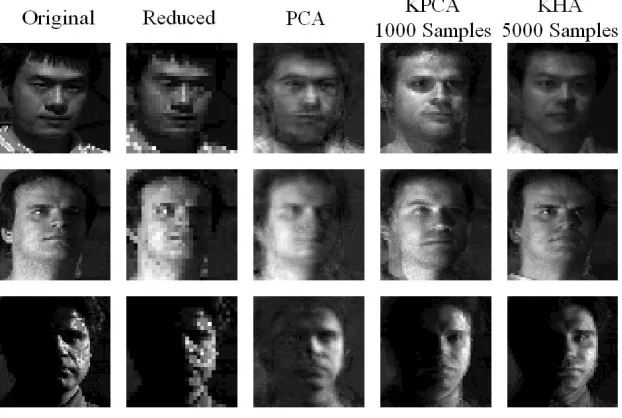
Interestingly, when the number of examples is small and the sampling of this manifold is sparse, this can have the consequence that the optimal KPCA (or KHA) reconstruction is an image that looks like the face of a wrong person. In a sense, this means that the errors performed by KPCA are errors along the manifold of faces. Figure 3 demonstrates this effect by comparing results from KPCA on 1000 example images (corresponding to a sparse sampling of the face manifold) and KHA on 5000 training images (denser sampling). As the examples shows, some of the misreconstructions that are made by KPCA due to the lack of training examples were corrected by the KHA using a large training set.

Hyperresolution of natural images. Figure 4 shows the first 40 principal components of 40,000 natural image

patches obtained from the KHA using a Gaussian kernel. The image database was obtained from [14]. Again,

Figure 3: Face reconstruction examples (from30×30resolution) obtained from KPCA and KHA trained on 1,000 and 5,000 examples, respectively. Occasional erroneous reconstruction of images indicates that KPCA requires a large amount of data to properly sample the underlying structure.

Figure 4: The first 40 kernel principal components of 40,000 (14×14)-sized patches of natural images obtained from the KHA using a Gaussian kernel withσ= 40.

a direct application of KPCA is not feasible for this large dataset. The plausibility of the obtained principal components can be demonstrated by increasing the size of the Gaussian kernel such that the distance metric of the corresponding RKHS becomes more and more similar to that of input space [2]. As can be seen in Fig. 4, the principal components approach those of linear PCA [4] as expected.

a b

c d

e f

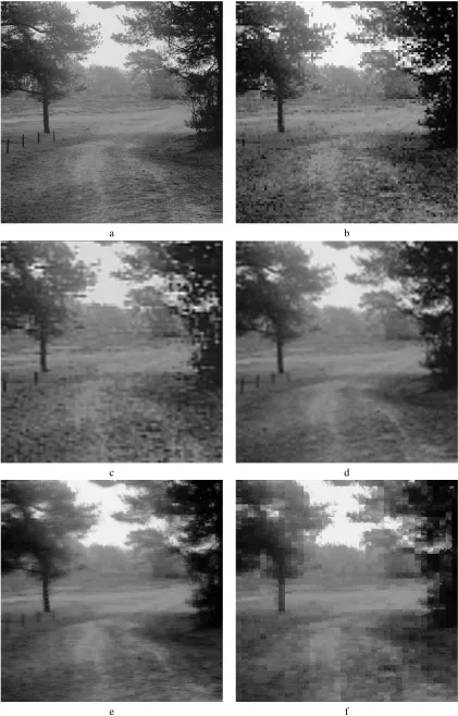
Figure 5: Example of natural image hyperresolution: a. original image of resolution400×400, b. low resolution image

(100×100)stretched to400×400, c. PCA reconstruction, d. bilinear interpolation, e. KPCA reconstruction with overlapping windows, and f. block-wise KPCA reconstruction.

5

Discussion

This paper formulates the KHA, a method for the efficient estimation of the principal components in an RKHS. As a kernelization of the GHA, the KHA allows for performing KPCA without storing the kernel matrix, such that large datasets of high dimensionality can be processed. This property makes the KHA particularly suitable for applications in statistical image hyperresolution. The images reconstructed by the KHA appear to be more realistic than those obtained by using linear PCA since the nonlinear principal components capture also part of the higher-order statistics of the input.

The time and memory complexity for each iteration of KHA isO(r×l×N)andO(r×l+l×N), respectively, wherer, l, and N are the number of principal components to be computed, the number of examples, and the dimensionality of input space, respectively.6 This rather high time complexity can be lowered by precomputing and storing the whole or part of the kernel matrix. When we store the entire kernel matrix, as KPCA does, the time complexity reduces toO(r×l). The number of iterations for the convergence of KHA depends on the number and characteristic of data. For superresolution experiments, iteration finishes when the squared distance between two solutions from consecutive iterations is larger than a given threshold. It took around 40 and 120 iterations for face and natural image hyperresolution experiments, respectively.

Since KHA assumes a finite number of examples, it is not a true online algorithm. However, many practical problems can be processed in batch mode (i.e., all the patterns are known in advance and the number of them is finite), but, it might be still useful to have an algorithm for applications where the patterns are not known in advance and are time-varying such that KPCA cannot be applied. Some issues regarding online applications are discussed in appendix.

A

Appendix: online kernel Hebbian algorithm

The proof in Section 3.2 does not draw any conclusion on the convergence properties of KHA when the number of independent samples inF is infinite. Naturally, this property depends not only on the characteristics of the underlying data but also on the RKHS concerned. A representative example of these spaces is the one induced by a Gaussian kernel where all different patterns are independent. Convergence of an algorithm in this true online problem might be of more theoretical interest, however, it is simply computationally infeasible as in this case the solutions are represented only based on an infinite number of samples. Still, much practical concern lies in applications where the sample set is not known in advance or the environment is not stationary.

This section present a modification of the batch type algorithm for this semi-online problem where the number of data points are finite but they are not known in advance or nonstationary. Two issues arise from this online setting: 1. To guarantee the nonorthogonality ofa(0)andq(Section. 3.3.3); 2. To estimate the center of data in online;

A.1 On the nonorthogonality condition of the initial solution

It should be noted from the original formulation of GHA in RKHS (7) that when the pattern presented at timet

is orthogonal to the solutionwi(t), the outputyibecomes zero, and accordinglywiwill not change. In general,

according to the rule (7),wi(t)cannot move into the direction orthogonal to itself. This implies that if the eigen-vectorvihappens to be orthogonal towi(t)att,wi(t)will not be updated in the direction ofvi. If this is true for

all timet, (i.e., all patterns contained in the training set are orthogonal either to thevior to thewi), then clearly wi(t)will not converge tovi. As a consequence, it is a prerequisite for the convergence thatwi(t)should not be

orthogonal tovifor all timest. Actually, this condition is equivalent to the nonorthogonality ofqiandai(t)in the

dual space since

wi·vi = a>i ΦΦ

>_q

i = a>i Kqi

= (

l

X

k=1

λkχkqi)>qi = λiχi,

where the third equality comes from (23). This is exactly why it is assumed thatχi6= 0during the stability analysis

of (20). From this dual representation, it is evident that for the batch problem, this condition can be satisfied with

6_¯

probability 1 by simply initializingai(0)randomly. However, this cannot be guaranteed for online learning since the examples are not known in advance and accordingly,ai(0)will in general not be contained in the span of the training sample. Furthermore we do not have any method to directly manipulatewi(0)inF. Accordingly, we cannot guarantee this condition in general RKHSs.

Instead we will provide a practical way to satisfy the condition for the most commonly used three kernels (Gaussian kernels, polynomial kernels, and tangent hyperbolic kernels). If we randomly choose a vectorxi(0)in

RN and initializewi(0)withΦ(xi(0)), then

wi(0)·vi = Φ(xi(0))·vi = Φ(xi(0))Φ>qi

= X

k=1

qikk(xi(0),xk).

Accordingly, in this case the orthogonality depends on the type of the kernel and is not always satisfied. However, for the Gaussian, polynomial, and tangent hyperbolic kernels, this initialization method is enough to ensure that

wi(0)·vi6= 0since

1. The output of an even polynomial kernel (k(x,y) = (x·y)p_{) is zero if and only if the inner product of two}

inputxandyin the input space is zero. For odd polynomial kernels (k(x,y) = (x·y+c)p_{), the zero output}

occurs only ifx·y=−c;

2. The output of a Gaussian kernel (k(x,y) = exp(− 1

2σ2kx−yk

2_{)) is not zero for a fixedσand boundedx}

andyin the input space;

3. Similar to the case of odd polynomial kernel, the output of a tangent hyperbolic kernel (k(x,y) = tanh(x·

y−b)) is zero if and only ifx·y=b.

For the case of 1 and 3, random selection ofx(0)in the input space yieldsk(x(0),xk)6= 0inFwith probability

1. Restricting the input data in a bounded domain guarantees this for the second case. Furthermore for each kernel type, ifx(0)is chosen at random, eachk(x(0),xl)is also random. this assures the nonorthogonality with probability 1.

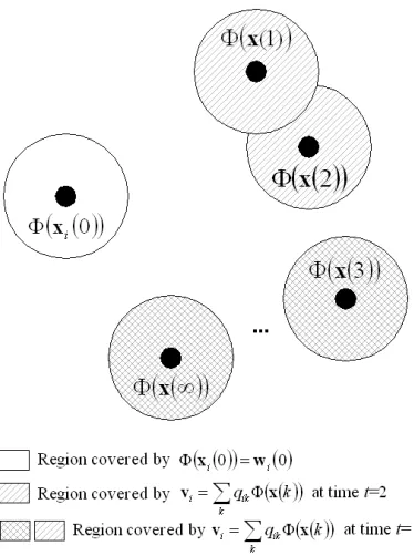
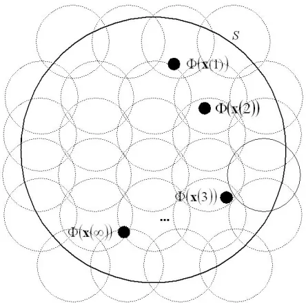
Actually, for Gaussian kernels with very smallσ, this initialization method does not guarantee the nonorthogo-nality in the real world (e.g., digital computers with limited precision). In this case, two arbitrary mapped patterns inF, which are far from each other in the input space would be regarded as orthogonal. This implies that there is a possibility thatk(xi(0),xk) = 0, for allk(Figure 6). Furthermore, since all patterns are independent, the eigenvector generally has to be expanded in all the examples. This implies thatwi(0)should be nonorthogonal to all the data points in order to guarantee convergence. However, if all the patterns in input space are bounded in a ballSwhich is the case in many practical applications, we can still satisfy this condition by constructingwi(0)as a linear combination of the mapped patterns, e,g., sampled inSat a small enough interval (Figure 7).

It should be noted that the above discussion is still valid for non-stationary environments, i.e.,vi is a

time-varying vector. In this case, the orthogonality condition ensures not the convergence but the tracking capability of the algorithm with the additional condition that the presentation of the patterns is fast enough to keep track of the change in the environment. In this case,η(t)should not tend to zero but to a small constant.

A.2 Kernelized update rule

The basic algorithm is the same as in (11), except that wi(0) = Φ(xi(0))with randomly chosen xi(0)(i.e.,

a(0)i0= 1anda(0)ij = 0forj >0) anda(t)ij= 0for allj > t. Then, we get the component-wise update rule:

aij(t+ 1) =

_{ηyi(t) if J(t) =j} aij(t)−ηyi(t)P

i

k=1akj(t)yk(t) otherwise,

where

yi(t) = t−1

X

k=1

ai(t)Φ(x(k))>Φ(x(t)) = t−1

X

k=1

aik(t)k(x(k),x(t)).

It should be noted that for online caseJ(t) =tand accordingly, the dimensionality of solution vectoraincreases proportionally tot.

Figure 6: Example of non-convergence of the online algorithm for a Gaussian kernel: Small black circles represent the locations of patterns in the input space while the large circles around them show the non-orthogonal regions. Gray circles show the region covered byvi. The white circle is the region covered bywi(0). If two regions covered bywi(0)andvido not overlap each

other, then they are orthogonal.

A.3 Centering data

Centering can be done by subtracting the sample mean from all patterns. Since this sample mean is not available for the online problem, we estimate at each time step the mean based only on the available data. In this case a pattern presented at timet(Φ(x(t))) is replaced by

e

Φ(x(t))= Φ(. x(t))−Φ(x(t)), (14)

whereΦ(x(t))is the estimated mean at timet−1: Φ(x(t)) = 1_tPt−1

k=1Φ(x(k)). Now,wandyare represented

based on the new centered expansions as7

wi(t) = t−1

X

k=1

aik(t)Φ(e x(k))

= t−1

X

k=1

aik(t) Φ(x(k))−1

t

t−1

X

l=0

Φ(x(l)))

! ,

7

Figure 7: Example of initializingwi(0)for a Gaussian kernel: Sampling points are not depicted. Instead, non-orthogonal regions are marked with dotted circles. If the sampling interval is small enough so that these regions coverS, thenwi(0)

cannot be not orthogonal to all the data points withinS.

wherewi(0) = Φ(xi(0))and

yi(t) = Φ(e x(t))·

t−1

X

k=1

aik(t)Φ(e x(k))

= t−1

X

k=0

aik(t)k(x(t),x(k))− 1

t "_t−1

X

k=0

aik(t) t−1

X

l=0

k(x(l),x(k))

!#

−1

t

t−1

X

k=0

k(x(t),x(k))

! t−1

X

l=0

ail(t)

!

+ 1

t2

 

t−1

X

k,l=0

k(x(k),x(l))

 

t−1

X

m=0

aim(t)

!

. (15)

Then, a new update rule (in component-wise form) based on (27)-(28) is obtained as

t

X

k=0

aik(t+ 1) Φ(x(k))− 1

t+ 1 t

X

l=0

Φ(x(l))

!

= t−1

X

k=0

"

aik(t)−ηyi(t) i

X

l=1

alk(t)yl(t)

!

Φ(x(k))−1

t

t−1

X

l=0

Φ(x(l))

!#

+ηyi(t) Φ(x(t))−1

t

t−1

X

l=0

Φ(x(l))

!

, (16)

the solution of which can be obtained from

aik(t+ 1) =

(

ηyi(t) +1_thPt−1

k=0(aik(t)−ηyi(t)

Pr

l=1alk(t)yl(t)) +ηyr(t)

i

if k=t aik(t)−ηyi(t)Pr

l=1alk(t)yl(t) otherwise.

(17)

For the computation ofy(t),Pt−1

k,l=0k(x(k),x(l))and

Pt−1

k=0k(x(k),x(i))are updated only fort−1.

Accord-ingly the time complexity of each step isO(r×t×N).

Acknowledgments. The authors greatly profited from discussions with A. Gretton, M. Hein, and G. Bakır.

References

[1] B. Sch¨olkopf, A. Smola, and K. M¨uller. Nonlinear component analysis as a kernel eigenvalue problem. Neural Compu-tation, 10(5):1299–1319, 1998.

[2] B. Sch¨olkopf and A. Smola. Learning with Kernels. MIT Press, Cambridge, MA, 2002.

[3] E. Oja. A simplified neuron model as a principal component analyzer. Journal of Mathematical Biology, 15:267–273, 1982.

[4] T. D. Sanger. Optimal unsupervised learning in a single-layer linear feedforward neural netowork. Neural Networks, 12:459–473, 1989.

[5] S. Mika, B. Sch¨olkopf, A. J. Smola, K.-R. M¨uller, M. Scholz, and G. R¨atsch. Kernel PCA and de-noising in feature spaces. In M. S. Kearns, S. A. Solla, and D. A. Cohn, editors, Advances in Neural Information Processing Systems 11, pages 536–542, Cambridge, MA, 1999. MIT Press.

[6] L. Ljung. Analysis of recursive stochastic algorithms. IEEE Trans. Automatic Control, 22(4):551–575, 1977.

[7] S. Haykin. Neural Networks: A Comprehensive Foundation. Prentice Hall, New Jersey, 2nd edition, 1999.

[8] D. J. Field. What is the goal of sensory coding? Neural Computation, 6:559–601, 1994.

[9] C. J. C. Burges. Simplified support vector decision rules. In L. Saitta, editor, Proceedings of the 13th International Conference on Machine Learning, pages 71–77, San Mateo, CA, 1996. Morgan Kaufmann.

[10] J. T. Kwok and I. W. Tsang. Finding the pre-images in kernel principal component analysis. 6th Annual Workshop On Kernel Machines, Whistler, Canada, 2002, poster available at http://www.cs.ust.hk/∼jamesk/kernels.html.

[11] F. M. Candocia. A unified superresolution approach for optical and synthetic aperture radar images. PhD thesis, Univ. of Florida, Grainesville, 1998.

[12] A. S. Georghiades, P. N. Belhumeur, and D. J. Kriegman. From few to many: illumination cone models for face recogni-tion under variable lighting and pose. IEEE Trans. Pattern Analalysis and Machine Intelligence, 23(6):643–660, 2001.

[13] S. Mika, G. R¨atsch, J. Weston, B. Sch¨olkopf, and K.-R. M¨uller. Fisher discriminant analysis with kernels. In Y.-H. Hu, J. Larsen, E. Wilson, and S. Douglas, editors, Neural Networks for Signal Processing IX, pages 41–48. IEEE, 1999.