Munich Personal RePEc Archive
An Econometric Analysis of Aggregate
Outbound Tourism Demand of Turkey
Halicioglu, Ferda
Department of Economics, Yeditepe University
2008
Online at
https://mpra.ub.uni-muenchen.de/6765/
Presented at the 6th DeHaan Tourism Management Conference: “The Economics of Tourism”, organized by the Christel DeHaan Tourism and Travel Research Institute, Nottingham University Business School
Nottingham-UK, 18th December 2007
An Econometric Analysis of Aggregate Outbound Tourism Demand of Turkey
Abstract
This study attempts to examine empirically aggregate tourism outflows in the case of Turkey using the time series data for the period 1970-2005. As far as this article is concerned, there exists no previous empirical work dealing with the tourist outflows from Turkey. The previous tourism studies in the case of Turkey, by and large, focus on the inbound tourism demand analyses. As a developing country and an important tourism destination, Turkey has also been a significant source for generating a substantial number of tourists in recent years. Therefore, the tourist outflows from Turkey deserve to be analysed empirically too.
The total tourist outflows from Turkey are related to real income and relative prices. The bounds testing to cointegration procedure proposed by Pesaran et al. (2001) is employed to compute the short and long-run elasticities of income and relative prices. An augmented form of Granger causality analysis is conducted amongst the variables of outbound tourist flows, income and relative prices to determine the direction of causality. In the long-run, causality runs interactively through the error correction term from income and relative prices to outbound tourist flows. However, in the short-run, causality runs only from income to outbound tourism flows. The aggregate tourism outflows equation is also checked for the parameter stability via the tests of cumulative sum (CUSUM) and cumulative sum of the squares (CUSUMSQ).
The empirical results suggest that income is the most significant variable in explaining the total tourist outflows from Turkey and there exists a stable outbound tourism demand function. The results also provide important policy recommendations.
Keywords: outbound tourism demand; cointegration; Granger causality; stability
tests; Turkey.
Correspondence to:
Ferda HALICIOGLU
Department of Economics Yeditepe University 34755 Istanbul Turkey
e-mail: fhalicioglu@yeditepe.edu.tr
Introduction
Outbound tourism in developing countries is regarded as a waste of valuable foreign reserves. Therefore, the authorities tend to restrict the outbound tourism demand via different forms of obstacles and policies, such as excess exit taxes, restrictions on issuing passports, limiting the amount of foreign currency to take abroad and multiple rates for the different purposes of foreign country visits. All these outbound tourism restrictions are aimed at preserving the foreign reserves for essential imports and foreign debt reductions. Turkey also resorted to the outbound demand restriction policies until the 1980s because Turkey pursued an import substitution policy as a development strategy until 1980. However, this development policy failed in the late 1970s causing massive bottlenecks in industries and foreign reserves deficits. In the last three decades, Turkey adopted the export-led growth development policy with the implementation of several major economic reforms in the fields of foreign trade, monetary and fiscal institutions, competition, state public enterprises, privatization, FDI, etc. The major aims of these economic reforms are to increase the efficiency of the economic resources and, hence, to close the economic development gap between Turkey and the developed countries. As of 2005, Turkey ranked the 17th biggest economy in the World with a population of over 73 million. Turkey’s economic integration into the world economy has been growing at a rapid rate since the early 1980s. To this end, the openness ratio, which is measured broadly as total imports and exports to gross domestic product, increased from 8.37% in 1970, to 15.51% in 1980 and to 46.4% in 2005. Although, the average per capita income is far below that of the developed countries, the real per capita rose to $ 3390 in 2005, from $1896 in 1980 and from $1650 in 19701. Easing the travelling restrictions abroad and the relatively faster economic development in Turkey have stimulated significantly the outbound tourist demand since the 1980s. As a consequence, the outbound tourism demand increased from 515,000 people with an expenditure of $12 million in 1970, to 1.65 million people with an expenditure of $104 million in 1980 and to 8.02 million people with an expenditure of $ 2.87 billion in 2005. The share of tourism expenditures in GDP appears to be very minimal, which is only 0.77% in 2005. These tourism expenditure ratios are 0.06% and 0.14% for 1970 and 1980, respectively. Nevertheless, the average growth rate of outbound tourism demand in the period of 1970-2005 is 9.38% whilst the real GDP growth in the same period is just 4.06%, indicating that there exists a substantially strong outbound tourism demand2. It seems that the current upward trend in the outbound tourism demand is likely to continue to grow faster, as Turkey becomes a full member of the European Union in the next decade.
Tourism demand models have been used extensively to analyse the demand behaviour and demand management issues in addition to forecast the future levels of tourism demand. The empirical estimates of income and relative price elasticities have particular relevance for designing appropriate income and pricing policies in the tourism sector.
1 These macroeconomic figures are obtained from
international financial statistics of IMF. The ratios are my own calculations from the same source.
2
There is extensive literature examining the tourism demand functions in the context of developing and developed countries using the single and multivariate cointegration techniques of the 1980s and 1990s. The results and implications of these studies clearly depend on the underlying variables, the econometric methods, data frequency, and the development stage of a country. Crouch (1994), Lim (1997), and Li et al. (2005) provide very comprehensive surveys of empirical tourism demand studies for the last four decades. These surveys reveal that most of the existing studies tend to use the tourist arrivals/departures and tourism revenues/expenditures as a dependent variable. The surveys also point out that the most widely used explanatory variables are income and price/relative prices. The theoretical basis for the selection of these explanatory variables is related to the consumer theory. However, many empirical studies also use additional explanatory variables ranging from transportation costs to time trends. The tourism demand equations are generally estimated in double logarithmic forms so that researchers obtain a direct estimate of elasticity of the dependent variable with respect to the explanatory variables. Recent econometric studies appear to present both the short-run and long-run estimates of the explanatory variables.
A large number of empirical papers on international tourism demand are found in the literature and are divided into two main categories.
The first category consists of studies that use modern time series and cointegration techniques in an attempt to model and forecast the dependent variable between one or several pairs of countries. See, for example, Kulendran (1996), Wong (1997), Kim and Song (1998), Kulendran and Witt (2001), Seddighi and Theocharous (2002), Song et al. (2003) and Dritsakis (2004), Charalambos (2006), and Li et al. (2006). The second category includes papers that estimate the determinants of international tourism demand using classical multivariate regressions. For a detailed survey of this literature, see Crouch (1994), Witt and Witt (1995), and Lim (1997).
The vast majority of international tourism demand studies are based on the inbound of tourist flows rather than the outbound tourist flows. However, a few recent studies on international tourism demand have presented empirical estimations of outbound tourism demand, see for example Song et al. (2000) for UK; Lim (2004) for Korea and Coshall (2006) for UK.
On researching the literature, one finds that there exist several empirical research studies dealing with the inbound tourism demand for Turkey using both the traditional and modern econometric techniques; see for example, Uysal and Crompton (1984),
Var et al. (1990), Ulengin (1995), Icoz et al. (1998), Akis (1998), Akal (2004), and
Halicioglu (2004). However, no study has attempted to model the outbound tourism demand for Turkey. Thus, this study seizes the opportunity to fill the gap in the literature.
see for example Kumar (2004) for Fiji; Halicioglu (2004) for Turkey; and Mervar and Payne (2007) for Croatia.
The objectives of this study are as follows: i) to estimate the income and relative price elasticities of the outbound tourism demand both in the short-run and long-run using the ARDL approach to cointegration; ii) to establish the direction of causal relationships between outbound tourism demand, income and relative prices; and iii) to implement parameter stability tests of Brown et al. (1975) to ascertain stability or instability in the outbound tourism demand function.
The remainder of this paper is organized as follows: the next section describes the study’s model and methodology. The third section discusses the empirical results, and the last section concludes.
Model and econometric methodology
Following the empirical literature in tourism economics, an aggregate outbound tourism demand regression model for Turkey in double logarithmic form is constructed as:
t t t
t a a y a p
f = 0 + 1 + 2 +ε (1)
where ft is aggregate tourist flows from Turkey, yt is real aggregate income, pt is
exchange rate adjusted relative prices and εt is the regression error term .
As for the expected signs in equation (1), one expects that because higher real income should result in greater economic activity and stimulate outbound tourism demand. The aforementioned empirical tourism demand surveys indicate that income elasticity estimates vary a great deal, but generally exceed unity and below 2.0 confirming that international travel is a luxury item.
0
1 >
a
The coefficient of the exchange rate adjusted relative price levels is expected to be less than zero for the usual economic reasons, therefore, a2 <0. The estimation results found in the tourism demand surveys regarding prices are rather uneven since there seems to be no agreement about the appropriate range of this coefficient. Estimated price elasticities vary dramatically both within and across papers. For example, they are in the range of –0.05 to –6.36.
the model in question are estimated simultaneously; iii) the ARDL approach to testing for the existence of a long-run relationship between the variables in levels is applicable irrespective of whether the underlying regressors are purely I(0), purely
I(1), or fractionally integrated; iv) the small sample properties of the bounds testing approach are far superior to that of multivariate cointegration, as argued in Narayan (2005).
An ARDL representation of equation (1) is formulated as follows:
t t t t m i m i m i i t i i t i i t i
t a a f a y a p a f a y a p v
f = + Δ + Δ + Δ + + + +
Δ − − −
= − = − = −
∑
∑
∑
4 1 5 1 6 11 0 0
3 2
1
0 (2)
Given that Pesaran et al. cointegration approach is a relatively recent development in the econometric time series literature, a brief outline of this procedure is presented as follows. The bounds testing procedure is based on the F or Wald-statistics and is the first stage of the ARDL cointegration method. Accordingly, a joint significance test that implies no cointegration hypothesis, (H0:a4 =a5 =a6 =0), against the
alternative hypothesis, (H1:a4 ≠a5 ≠a6 ≠0) should be performed for equation (2).
The F test used for this procedure has a non-standard distribution. Thus, Pesaran et al. compute two sets of critical values for a given significance level with and without a time trend. One set assumes that all variables are I(0) and the other set assumes they are all I(1). If the computed F-statistic exceeds the upper critical bounds value, then the H0 is rejected. If the F-statistic falls into the bounds then the test becomes inconclusive. Lastly, if the F-statistic is below the lower critical bounds value, it implies no cointegration. This study, however, adopts the critical values of Narayan (2005) for the bounds F-test rather than Pesaran et al. (2001). As discussed in Narayan (2005) given relatively a small sample size in this study (36 observations), the critical values produced by Narayan (2005) are more appropriate than that of Pesaran et al. (2001).
Once a long-run relationship has been established, equation (2) is estimated using an appropriate lag selection criterion. At the second stage of the ARDL cointegration procedure, it is also possible to perform a parameter stability test for the selected ARDL representation of the error correction model.
A general error correction model (ECM) of equation (2) is formulated as follows:
t t m i m i m i i t i i t i i t i
t a a f a y a p EC
f = + Δ + Δ + Δ +λ +μ
Δ −
= − = − = −
∑
∑
∑
11 0 0
3 2
1
0 (3)
where λ is the speed of adjustment parameter and ECt-1 is the residuals that are obtained from the estimated cointegration model of equation (1).
involving the error correction term is formulated in a multivariate pth order vector error correction model.
[
]
⎥ ⎥ ⎥ ⎦ ⎤ ⎢ ⎢ ⎢ ⎣ ⎡ + ⎥ ⎥ ⎥ ⎦ ⎤ ⎢ ⎢ ⎢ ⎣ ⎡ + ⎥ ⎥ ⎥ ⎦ ⎤ ⎢ ⎢ ⎢ ⎣ ⎡ ⎥ ⎥ ⎥ ⎦ ⎤ ⎢ ⎢ ⎢ ⎣ ⎡ − + ⎥ ⎥ ⎥ ⎦ ⎤ ⎢ ⎢ ⎢ ⎣ ⎡ = ⎥ ⎥ ⎥ ⎦ ⎤ ⎢ ⎢ ⎢ ⎣ ⎡ − − − − − =∑
t t t t i t i t i t i i i i i i i i i i i i p i t t t EC p y f d d d d d d d d d d d d L c c c p y f L 3 2 1 1 3 2 1 34 33 32 31 24 23 22 21 14 13 12 11 1 3 2 1 ) 1 ( ) 1 ( ω ω ω λ λ λ (4) ) 1( −L is the lag operator. ECt-1 is the error correction term, which is obtained from the long-run relationship described in equation (1), and it is not included in equation (4) if one finds no cointegration amongst the vector in question. The Granger causality test may be applied to equation (4) as follows: i) by checking statistical significance of the lagged differences of the variables for each vector; this is a measure of short-run causality; and ii) by examining statistical significance of the error-correction term for the vector that there exists a long-run relationship. As a passing note, one should reveal that equation (3) and (4) do not represent competing error-correction models because equation (3) may result in different lag structures on each regressors at the actual estimation stage; see Pesaran et al. (2001) for details and its mathematical derivation. All error-correction vectors in equation (4) are estimated with the same lag structure that is determined in unrestricted VAR framework; see for example, Narayan and Singh (2006). This study utilizes the latter procedure.
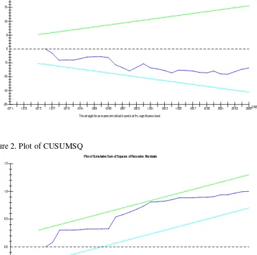
The existence of a cointegration derived from equation (2) does not necessarily imply that the estimated coefficients are stable, as argued in Bahmani-Oskooee and Chomsisengphet (2002). The stability of coefficients of regression equations are, by and large, tested by means of Chow (1960), Brown et al. (1975), Hansen (1992), and Hansen and Johansen (1993). The Chow stability test requires a priori knowledge of structural breaks in the estimation period and its shortcomings are well documented, see for example Gujarati (2003). In Hansen (1992) and Hansen and Johansen (1993) procedures, stability tests require I(1) variables and they check the long-run parameter constancy without incorporating the short-run dynamics of a model into the testing - as discussed in Bahmani-Oskooee and Chomsisengphet (2002). Hence, stability tests of Brown et al. (1975), which are also known as cumulative sum (CUSUM) and cumulative sum of squares (CUSUMSQ) tests based on the recursive regression residuals, may be employed to that end. These tests also incorporate the short-run dynamics to the long-run through residuals. The CUSUM and CUSUMSQ statistics are updated recursively and plotted against the break points of the model. Provided that the plots of these statistics fall inside the critical bounds of 5% significance, one assumes that the coefficients of a given regression are stable. These tests are usually implemented by means of graphical representation.
Empirical results
Annual data over the period 1970-2005 were used to estimate equation (2) by the Pesaran et al. procedure. Data definition and sources of data are cited in the Appendix A.
Equation (2) was estimated in two stages. In the first stage of the ARDL procedure, the long-run relationship of equation (1) was established in two steps. Firstly, the order of lags on the first–differenced variables for equation (2) was obtained from unrestricted VAR by means of Akaike Information Criterion (AIC) and Schwarz Bayesian Criterion (SBC). The results of this stage are not displayed here to conserve space. Secondly, a bounds F test was applied to equation (2) in order to establish a long-run relationship between the variables.
Narayan and Smyth (2006) presents a detailed procedure to explain if one needs to implement the bounds F test with or without a time trend. It is possible that at the end of this testing procedure, one may end up with more than one possible cointegration relationship: one with a time trend and one without a time trend. As Narayan and Smyth (2006, p.116) argues that “in the spirit of the bounds test, model two with a time trend is invalid because for the model to be valid there should be only one long-run relationship”. In order to avoid a possible selection problem at this stage, one may follow the procedure of Bahmani-Oskooee and Goswami (2003) which sequentially test the long-run cointegration relationship in equation (2) on the basis of different lag lengths. This study adopts the second approach which implicitly assumes that equation (2) is free from a trend due to the differenced variables. In summary, the F tests indicate that there exists only one cointegrating relationship without a time trend in which the dependent variable is outbound tourism demand. The procedures of this stage and the results of the bounds F testing are outlined and presented in the Appendix B.
Given the existence of a long-run relationship, in the next step the ARDL cointegration procedure was implemented to estimate the parameters of equation (2) with maximum order of lag set to 2 to minimize the loss of degrees of freedom. This stage involves estimating the long-run and short-run coefficients of equations (1) and (2). In search of finding the optimal length of the level variables of the short-run coefficients, several lag selection criteria such as 2
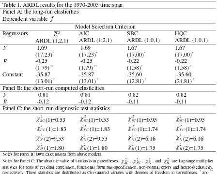
R , AIC, SBC and Hannan-Quinn Criterion (HQC) were utilized at this stage. The long-run results of equation (2) based on several lag criteria are reported in Panel A of Table 1 along with their appropriate ARDL models. The results from model selection criteria of 2
R and AIC are identical. Similarly, the results of SBC and HQC are exactly the same. As can be seen from Table 1, the long-run results are quite similar with regard to coefficient magnitudes and statistical significance. On the basis of estimated models, short-run income and relative price elasticities are computed, and the results are reported in Panel B of Table 1. The short-run elasticities, as expected, are smaller than the long-run values. However, the magnitudes of elasticities are very close in all the models.
Table 1. ARDL results for the 1970-2005 time span Panel A: the long-run elasticities
Dependent variable f
Model Selection Criterion
Regressors 2
R ARDL (1,2,1) AIC ARDL (1,2,1) SBC ARDL (1,0,1) HQC ARDL (1,0,1)
y 1.69
(17.23)* 1.69 (17.23)* 1.67 (17.00)* 1.67 (17.00)* p -0.25
(1.79) **
-0.25 (1.79) **
-0.22 (1.58)*
-0.22 (1.58) *
Constant -35.87 (13.01) *
-35.87 (13.01) *
-35.60 (12.81) *
-35.60 (21.81) *
Panel B: the short-run computed elasticities
y 0.81 0.81 0.82 0.82
p -0.12 -0.12 -0.11 -0.11
Panel C: the short-run diagnostic test statistics
2
SC
χ (1)=0.53 2
SC
χ (1)=0.53 2
SC χ (1)=0.95 2 FC χ (1)=1.83 2 N χ (2)=9.53 2 H χ (1)=1.80 2 FC
χ (1)=1.83 2
FC
χ (1)=1.74
2
N
χ (2)=9.53 2
N χ (2)=6.16 2 H χ (1)=1.75 2 SC χ (1)=0.95 2 FC χ (1)=1.74 2 N χ (2)=6.16 2 H χ (2)=1.75 2 H χ (1)=1.80
Notes for Panel B: Own calculations from above models.
Notes for Panel C: The absolute value of t-ratios is in parentheses. , , , and are Lagrange multiplier statistics for tests of residual correlation, functional form mis-specification, non-normal errors and heteroskedasticity, respectively. These statistics are distributed as Chi-squared variates with degrees of freedom in parentheses.
2 SC χ 2 FC χ 2 N χ 2 H χ
* and **
indicate 5 % and 10 % significance levels, respectively
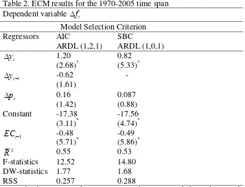
In search of finding the short-run dynamics of the above models, their error-correction representations were estimated as auxiliary models. The estimation results and the respective appropriate optimal lag length selection criteria with some selected diagnostics are displayed in Table 2. The error-correction models were only estimated in the case of AIC and SBC since the other model selection criteria displayed the identical results. Both the error-correction terms are statistically significant and their magnitudes are very close to each other. Considering the reported diagnostic test results and the statistical significance of the coefficients estimated in the long run and short-run, on average, the AIC model appears to be statistically more acceptable than the SBC criterion. The AIC model performs relatively better in terms of dynamics of the short-run variables, goodness of fit and RSS values. Therefore, it is quite plausible to accept the AIC based results as the preferred model for the evaluation of results and inference from there.
that the level of outbound tourism demand cannot be regulated extensively through price policies.
[image:10.595.86.443.185.458.2]The error-correction term is –0.48 with the expected sign, suggesting that when demand is above or below its equilibrium level, demand adjusts by almost 50% within the first year. The full convergence process to its equilibrium level takes after about two years. Thus, the speed of adjustment is significantly fast in the case of any shock to the outbound tourism demand equation.
Table 2. ECM results for the 1970-2005 time span Dependent variable Δft
Model Selection Criterion Regressors AIC
ARDL (1,2,1)
SBC
ARDL (1,0,1)
t
y
Δ 1.20
(2.68)*
0.82 (5.33)*
1 −
Δyt -0.62
(1.61)
-
t
p
Δ 0.16
(1.42)
0.087 (0.88) Constant -17.38
(3.11)*
-17.56 (4.74)*
1 −
t
EC -0.48
(5.71)*
-0.49 (5.86)*
2
R 0.55 0.53
F-statistics 12.52 14.80
DW-statistics 1.77 1.68
RSS 0.257 0.288
Notes: The absolute values of t-ratios are in parentheses. RSS stands for residual sum of squares. Since the AIC and HQC criteria produce exactly the same error correction results, the latter estimation, therefore, is not reported here. * and ** indicate 5 % and 10 % significance levels, respectively.
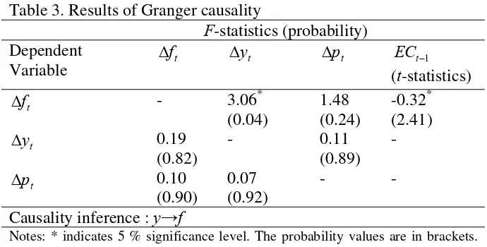
Having a cointegrating relationship among [ft, yt, pt] on the basis of the results of the
Table 3. Results of Granger causality
F-statistics (probability) Dependent
Variable t
f
Δ Δyt Δpt ECt−1
(t-statistics)
t
f
Δ - 3.06*
(0.04)
1.48 (0.24)
-0.32* (2.41)
t
y
Δ 0.19
(0.82)
- 0.11 (0.89)
-
t
p
Δ 0.10
(0.90)
0.07 (0.92)
- -
Causality inference : y→f
Notes: * indicates 5 % significance level. The probability values are in brackets. The optimal lag length is 2 and is based on SBC.
Figure 1. Plot of CUSUM
Plot of Cumulative Sum of Recursive Residuals
The straight lines represent critical bounds at 5% significance level -5
-10
-15
-20 0 5 10 15 20
[image:12.595.109.483.156.528.2]1971 1973 1975 1977 1979 1981 1983 1985 1987 1989 1991 1993 1995 1997 1999 2001 2003 20052005
Figure 2. Plot of CUSUMSQ
Plot of Cumulative Sum of Squares of Recursive Residuals
The straight lines represent critical bounds at 5% significance level -0.5
0.0 0.5 1.0 1.5
Conclusions
Like many developing countries, Turkey has been contributing to the growth of international tourism demand. The extent of this contribution in the coming years is expected to be more apparent once the travel restrictions such as harsh visa procedures imposed on Turkish citizens are lifted in the course of Turkey’s becoming a full member of the European Union. The number of Turkish people travelling abroad for holidays will double in less than a decade if the current average growth rate for the outbound tourism demand holds. The outbound tourism expenditures, however, will not be a significant burden in the foreign reserves since the share of the outbound tourism expenditures in GDP is rather low3. Thus, the tourism policies to design to restrict the outbound tourism demand may not produce the desired effects. In order to measure the extent of the economic policy decisions on the outbound tourism demand, this study computed the elasticities of the outbound tourism demand equation with respect to income and relative prices both in the short-run and long-run by employing the ARDL cointegration procedure. The computed ranges of elasticities are in line with the previous studies in the tourism demand literature. As expected, the long-run elasticities are greater than the short-run elasticities. These results may be utilized in managing the aggregate outbound tourism demand. For example, relatively low price elasticities in both the short-run and long-run indicate that the tourism policies to restrict outbound tourism demand would not be very effective, whilst the income policies will have a stronger impact on demand. The results of augmented Granger causality test suggest that the direction of causality runs interactively through the error-correction term from income and relative prices to the outbound tourism demand in the long-run. In the short-run, causality runs only from income to outbound tourism flows. Thus, the prediction of the level of the outbound tourism demand is possible by using income and relative prices variables. The parameter stability tests of the CUSUM and CUSUMSQ revealed that the outbound tourism demand equation is stable. Therefore, the suggested econometric model of the outbound tourism demand may be adopted for policy simulations and forecasting purposes.
3 The prediction of the total tourist outflows from Turkey is based on the average growth rate of the
Appendix A
Data definition and sources
All data are collected from International Financial Statistics of (IMF), Turkish Statistical Institute (TSI), and Ministry of Tourism and Culture of Turkey (MTCT),
f is total tourist outflows in thousands, in logarithm. The total tourist outflows data discontinued in the years of 1977, 1978 and 1979. The missing years were completed by extrapolation. Sources: TSI and MTCT.
y is real gross domestic product in thousands of Turkish Lira (TL), in logarithm. Gross domestic production is deflated by the consumer price index (CPI) of 2000=100. Source: IMF.
p is exchange rate adjusted relative prices between USA and Turkey, which is
measured as: ⎟⎟
⎠ ⎞ ⎜⎜
⎝ ⎛
× =
ER CPITurkey
CPIUSA
p , where CPIUSA is consumer price index of USA, CPITurkey is consumer price index of Turkey, and ER is the nominal exchange rates between USA and Turkey. Consumer price indexes are based on 2000=100. Source: IMF.
Appendix B
Bounds Test for Cointegration
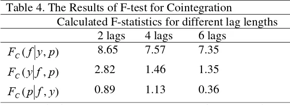
[image:14.595.84.377.606.713.2]A bounds F test was applied to equation (2) in order to test the existence of a long-run relationship by using lags from two to four following Bahmani-Oskooee and Goswami (2003), as they have shown that the results of this stage are sensitive to the order of VAR. Equation (2) was also estimated three more times in the same way but the dependent variable each time was replaced by one of the explanatory variables in search of other possible long-run relationship in any other form than it had already been described in equation (1). Summary results of bounds tests are presented in Table 4. Table 4 indicates only one plausible long-run relationship in which f is the dependent variable. Evidence of cointegration among variables also rules out the possibility of estimated relationship being “spurious”.
Table 4. The Results of F-test for Cointegration
Calculated F-statistics for different lag lengths 2 lags 4 lags 6 lags
) , (f y p
FC 8.65 7.57 7.35
) , (y f p
FC 2.82 1.46 1.35
) , (p f y
FC 0.89 1.13 0.36
References
Akal, M. (2004), ‘Forecasting Turkey’s tourism revenues by ARMAX model’
Tourism Management, Vol 25, No 5, pp 565-580.
Akis, S. (1998), ‘A Compact econometric model of tourism demand for Turkey’,
Tourism Management, Vol 19, No 1, pp 99-102.
Bahmani-Oskooee, M., and Chomsisengphet, S. (2002), ‘Stability of M2 demand functions in industrial countries’, Applied Economics, Vol 34, No 18, pp 2075-2083. Bahmani-Oskooee, M., and Goswami, G. G. (2003). ‘A disaggregated approach to test the J-curve phenomenon: Japan versus her major trading partners’. Journal of
Economics and Finance, Vol 27, No 1, pp 102-113.
Brown, R. L., Durbin, J., and Evans, J. M. (1975), ‘Techniques for testing the constancy of regression relations over time’, Journal of the Royal Statistical Society, SeriesB, Vol 37, No 2, pp 149-163.
Charalambos, L. (2006), ‘Income and expenditure in the tourism industry: time series evidence from Cyprus’, Tourism Economics, Vol 12, No 4, pp 603-617.
Chow, G. (1960), ‘Test of equality between sets of coefficients in two linear regressions’, Econometrica , Vol 28, No 3, pp 591-605.
Coshall, J. (2006), ‘Time series analyses of UK outbound travel by air’, Journal of
Travel Research, Vol 44, No 3, pp 335-347.
Crouch, I. (1994), ‘The study of international tourism demand: a survey of practice’,
Journal of Travel Research, Vol 32, No 4, pp 12-23.
Dritsakis, N. (2004) “Cointegration analysis of German and British tourism demand for Greece’, Tourism Management, Vol 25, No 1, pp 111-119.
Engle, R., and Granger, C. (1987), ‘Cointegration and error correction representation: estimation and testing’, Econometrica, Vol 55, No 2, pp 251-276. Gujarati, D. N. (2003), Basic Econometrics, 4th ed., McGraw Hill-Publishing, Boston. Halicioglu, F. (2004), ‘An ARDL model of aggregate tourism demand for Turkey’,
Global Business and Economic Review-Anthology, Vol 1, pp 614-623.
Hansen, B. E. (1992), ‘Tests for parameter instability in regressions with I(1) processes’, Journal of Business and Economic Statistics, Vol 10, No 3, pp 321-335. Hansen, H. and Johansen, S. (1993), Recursive Estimation in Cointegrated VAR
Models, Institute of Mathematical Statistics, preprint No.1, January, University of
Copenhagen, Copenhagen.
Icoz, O., T. Var, and Kozak, M. (1998), ‘Tourism demand in Turkey’, Annals of
Tourism Research, Vol 25, No1, pp 236-240.
IMF, International Financial Statistics, various issues, Washinghton DC.
Johansen, S. (1988), ‘Statistical analysis of cointegrating vectors’, Journal of
Economic Dynamics and Control, Vol 12, No 2/3, pp 231-254.
Johansen, S. and Juselius, K. (1990), ‘Maximum likelihood estimation and inference on cointegration–with application to the demand for money’, Oxford Bulletin of
Economics and Statistics, Vol 52, No 2, pp 169-210.
Johansen, S. (1996), Likelihood-Based Inference in Cointegrated Vector
Auto-Regressive Models, 2nd edn., Oxford University Press, Oxford.
Kim, S. and Song, H. (1998),‘Analysis of tourism demand in South Korea: a cointegration and error correction approach’, Tourism Economics, Vol 3, No 1, pp 25-41.
Kulendran, N. and Witt, S. F. (2001), ‘Cointegration versus least squares regression’,
Annals of Tourism Research, Vol 28, No 2, pp 291-311.
Kumar, N. P. (2004), ‘Fiji’s tourism demand: the ARDL approach to cointegration’,
Tourism Economics, Vol 10, No 2, pp 193-210.
Li, G., Song, H., and Witt, S. F. (2005) ‘Recent developments in econometric modelling and forecasting’, Journal of Travel Research, Vol 44, No 1, pp 82-89. Li, G., Wong, K. F., Song, H., and Witt, S. F. (2006), ‘Tourism demand forecasting: a time varying parameter error correction model’, Journal of Travel Research, Vol 45, No 2, pp 186-193.
Lim, C. (1997), ‘Review of international tourism demand models’, Annals of Tourism
Research, Vol 24, No 4, pp 835-849.
Lim, C. (2004), ‘The major determinants of Korean outbound travel to Australia’,
Mathematics and Computers in Simulation, Vol 64, No 3/4, pp 477-485.
Mervar, A and Payne, J. E. (2007), ‘Analysis of foreign demand for Croatian destinations: long-run elasticity estimates’, Tourism Economics, Vol 13, No 3, pp 407-420.
Ministry of Tourism and Culture of Turkey, annual tourism statistics, various issues, Ankara.
Narayan, P. K. (2005), ‘The Saving and investment nexus for China: evidence from cointegration tests’, Applied Economics, Vol 37, No 17, pp 1979-1990.
Narayan, P. K. and Smyth, R. (2006), “Higher education, real income and real investments in China: evidence from Granger causality tests’, Education Economics, Vol 14, No 1, pp 107-125.
Pesaran, M. H., Shin, Y., and Smith, R. J. (2001), ‘Bounds testing approaches to the analysis of level relationships’, Journal of Applied Econometrics, Vol 16, No 3, pp 289-326.
Phillips, P. and Hansen, B., (1990), ‘Statistical inference in instrumental variables regression with I(1) process’, Review of Economic Studies, Vol 57, No 1, pp 99-125. Seddighi, H. R. and Theocharous, A. L. (2002), ‘A model of tourism destination choice: a theoretical and empirical analysis’, Tourism Management, Vol 23, No 5, pp 475-487.
Song, H. and Li, G. (2008), ‘Tourism demand modeling and forecasting – a review of recent research’, Tourism Management, Vol 29, No 2, pp 203-220.
Song, H., Witt, S. F., and Jensen, T. C. (2003), ‘Tourism forecasting: accuracy of alternative econometric models’, International Journal of Forecasting, Vol 19, No 1, pp 123-141.
Song, H., Romilly, P., and Liu, X. (2000), ‘An empirical study of outbound tourism demand in the UK’, Applied Economics, Vol 32, No 5, pp 611-624.
Turkish Institute of Statistics, annual statistics year books, various issues, Ankara. Ulengin, B. (1995), ‘Factors affecting demand for international Tourist flows to Turkey’, Paper submitted for the 15th Annual Symposium on Forecasting, 4-7 June, Toronto, Canada.
Uysal, M. and Crompton, L. (1984), ‘Determinants of demand for international tourist flows to Turkey’, Tourism Management, Vol 5, No 4, pp 288-297.
Var, T., Mohammad, G., and Icoz, O. (1990), ‘Factors affecting international tourism demand for Turkey’, Annals of Tourism Research, Vol 17, No 3, pp 606-610.