Investment Under Uncertainty: A Theory

Munich Personal RePEc Archive

Investment Under Uncertainty: A

Theory

Mellati, Ali

Gokhale Institute of Politics and Economics

April 2008

Investment Under Uncertainty: A Theory

ALI MELLATI

alimellaty@gmail.com

GOKHALE INSTITUTE OF POLITICS AND ECONOMICS

BMCC ROAD, DECCAN GYMKHANA

PUNE - 411 004

INDIA

April, 2008

TELEPHONE: (+91 20) 25650287, 25654288/89, 25675008

FAX: (+91 20) 25652579

Website: http://www.gipe.ernet.in

Abstract

There must be a restricted time horizon within which investors trust their anticipations in an

uncertain condition. In this circumstance investors are concerned about what happens if the

worst condition (i.e. decreasing prices) occurs. A best-worst strategy in a discounted payback

period framework is applied to examine the effect of uncertainty on the time horizon and

investment. The model shows that increasing uncertainty will reduce the time horizon as well

as investment. Moreover, the calculated time horizon can be considered as a benchmark for

the adjusted payback period approach in finance.

Keywords: Uncertainty, Investment, Discounted payback period, best-worst strategy.

I. Introduction

Neo-classics assume identical definition for risk and uncertainty, while

post-Keynesians distinguish between them and criticize neo-classics for this presumption.

Post-Keynesians argue that how neo-classics maximize something about which there is no reliable

information. Furthermore, the effect of uncertainty on investment is not clear in the

neo-classical approach. The common methodology of neo-classics is that they try to examine the

effect of uncertainty on investment, optimized by maximization of future receipts, through its

effect on the some properties of the production function. Different presumptions about the

production function’s characteristics will lead to the contradictory consequences.

Post-Keynesians try to adapt a correct definition of uncertainty but they fail to show

how a higher level of uncertainty will affect investment. When uncertainty is defined as

something that we do not know anything about then it become impossible to examine it.

Neo-classics and post-Keynesians constitute two extremes. While neo-classics assume

that future is a perfect extension of the past, post-Keynesians assume that we are in an

absolutely chaotic unpredictable world so that the past can tell nothing about the future. It

seems that the real world is somewhere between these two extremes.

In this study I distinguish between risk and uncertainty but I assume a

quasi-predictable world. Corresponding to existing institutions there must be a limited time horizon

within which investors can rely on their information and their predictions. A new theory is

presented in the form of a different strategy for investment decision. Moreover, this theory

introduces a benchmark for the discounted payback period method in finance. It is concluded

that increasing uncertainty will reduce the investment. Section 1 dedicated to literature

II. Literature Review

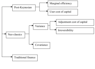
We can classify different theories of investment under uncertainty in three routes:

neo-classics, post-Keynesian and traditional finance. The classification of different theories of

investment under uncertainty has been presented in figure-11_{. They diverge through their}

different definitions of uncertainty and different assumptions about conditions in which the

investment decision is taken. The post-Keynesians and neo-classics differ essentially through

their definition of uncertainty. Neo-classical methods focus on uncertainty about the

components of the profit function (e.g. demand and price of output, costs etc.) where profit is

derived from process of production while traditional finance has focused on streams of profits

from securities (and not dividend) in stock markets.

Figure 1 Classification of the methods in dealing with uncertainty in investment theory.

1 _{This classification is an extension of John V. Leahy and Tom M. Whited (1996)}

Post-Keynesian

Neo-classics

Traditional finance

Marginal efficiency

User cost of capital

Adjustment cost of capital

Irreversibility Variance

Traditional finance- Likewise to the neo-classics, in traditional finance point of view,

price signals provide information about objective probabilities, and expectations can be

shaped through analysis of probabilities determined from past data. It treats expectations as a

determinant of gambling, and explains how we can evaluate it on the basis of a population

parameter estimated by a probability determined from a sample. Estimation of the frequency

distribution of the population can provide a reliable prediction about the future, because the

pattern of occurrence of events is assumed to be constant over time. We can then calculate

the expected value of a random variable and use it to make rational investment decisions to

maximize net wealth. In this method, probabilistic risk and uncertainty has been considered

synonymous. With regard to this definition, Modigliani and Miller (1958) have calculated the

market price associated with uncertain streams. Uncertainty is incorporated as a supplement

to the certain interest rate in the form of a risk premium in order to determine the cost of

capital. In order to maximize his wealth, a rational investor invests so that the marginal yield

of his capital is equal to the risk adjusted cost of capital. In this analysis more uncertainty will

lead to a higher risk premium and therefore higher cost of capital. Hence, investment will be

decreases.

Neo-classics- The neo-classical method takes in two separate routs: The first one,

which is denoted by Variance, considers a firm by itself divorced from the existence of other

projects and emphasizes the variance of some component of environment of a project (e.g.

demand, costs, etc.) as uncertainty. The second, which is represented by covariance,

emphasizes on the relationship between one firm with other firms in a market and relates the

uncertainty to the covariance of their returns. Neo-classical methods, which emphasize on the

variance as a proxy of uncertainty, diverge in two separate channels again. According to Abel

The firm’s investment decision becomes an interesting dynamic problem, in

which anticipations about the future economic environment affect current investment,

when frictions prevent instantaneous and costless adjustment of the capital stock.

Literatures focused on two types of frictions: adjustment costs and irreversibility.

Adjustment-cost literatures are based on the study of Eisner and Strotz (1963). They

assume that firms face extra costs of adjusting their capital stock and these costs are a convex

function of the rate of change of the capital stock of the firm. This implies that it is costly for

a firm to increase or decrease its capital stock, and that the marginal adjustment cost is

increasing in the size of the adjustment. Studies with this assumption have been lead to a

positive relationship between uncertainty and investment (Hartman, 1972, 1973; Abel, 1983).

The irreversibility literatures are traced back to Arrow (1968). He argues that:

There will be many situations in which the sale of capital goods cannot be

accomplished at the same price as their purchase…For simplicity, we will make the

extreme assumption that resale of capital good is impossible, so that gross investment

is constrained to be non- negative.

Contrary to the costs-adjustment method, irreversibility predicts a concave marginal revenue

product of capital. According to Leahy and Whited (1996) it makes returns to investment

asymmetric:

If the future returns out to be worse than expected, the marginal revenue

product of capital falls and the investor is stuck with lower returns. If prospects

improve, the incentive is to invest more, thereby limiting the rise in the marginal

revenue product of capital. This asymmetry implies that the marginal revenue product

of capital is a concave function of wages and prices.

The effect of uncertainty on investment under the assumption of irreversibility is not clear. It

1992). Abel and Eberly (1996) argue that the relationship could be negative even when the

capital is costly reversible. But when the construction of a project lasts for some periods this

relationship can be positive (Bar-Ilan and Strange ,1996). For an ongoing firm the effect of

uncertainty on long –run investment is not clear (Abel and Eberly ,1995).

Craine (1989) tries to examine the effect of uncertainty on the allocation of capital in

a simple general equilibrium model. He measures uncertainty as the covariance between the

riskless discount factor and the firm’s return factor. He concludes that a mean preserving

spread in the distribution of the state of nature that affects firm’s technologies or household’s

preferences has no effect on aggregate investment, but it alters the allocation of capital and

labor among technologies. Therefore, the share of capital devoted to less risky technologies

increases.

Post-Keynesians- Keynes and post-Keynesians separate their approach by a different

definition of uncertainty. As Kregel (1998) argues:

An obvious criticism is that the uncertainty faced in real life is unlike the

uncertainty over outcomes of games of chance, because there is no possibility of

random sampling with replacement. …if the underlying population is not constant,

there is no possibility of forming a sample statistic based on expectation of the

frequency distribution, irrespective of whether there is sampling with replacement at

a given point in time and no expectation of the likely occurrence of specific

realizations can be formed on the basis of standard statistical methods.

Each event in time occurs due to a decision of an agent when he is confronted with

what Kregel (1999) calls (quoted from Frank Knight) a ‘unique situation’. Furthermore,

individuals might make a mistake either due to inadequacy of information or due to their

limited computational ability to deal with a large number of possibilities. As, agents cannot

1996).Arestis concludes that the past is immutable and the future is blurred and unknowable.

Probability analysis is reliable when we have a statistic process in which the average

calculated from the past events cannot persistently different from the time average of future

outcomes (Davidson, 1991). We can have this process when economic conditions are

produced by natural laws. According to Kregel and Nasica (1999):

If there are ‘natural’ or ‘objective’ laws producing current economic

conditions, independently of agents’ expectations, then there will be objective

probability distributions which can be estimated with increasing certain by standard

statistical procedures. But the real point of difficulty concerned the existence of the

natural law, the specification of the objective process generating the results, which

expectations would reflect, not with the process of predicting them.

Because economic decisions are taken on the basis of human expectations, relevant

variables might not be governed entirely by a natural law. Thus, we cannot predict the future

expectations on the basis of past observation. Thus, Davidson (1991) explains that the

objective probabilities and rational expectations may be reasonable for estimation in some

area of economic decision-making but it cannot be seen as a general theory. Hence we can

define an uncertain situation as a condition about which we do not know anything about it

and it is distinctly different from a risky situation, which is characterized by a probability

distribution over a few events. In this condition, rationality of the agent is expresses through

the formulation of probability which is based on uncertain information and doubtful

arguments, or the depiction of animal spirits (Kregel, 1987).

Kregel (1987) expresses rationality on the lines suggested by Keynes by saying that

rational agent responds to uncertainty through use of money as a store of value where the

price of money is determined by the effect of uncertainty on liquidity preference. Davidson

money and law of civil contracts: in an uncertain world where liabilities are enforceable only

in terms of money, entrepreneurs have to form sensible expectations about the certainty of

future cash flows. Entrepreneurs limit their contracts and liabilities to what they believe their

liquidity position can survive. They do not make any significant decisions involving real

resource commitments until they are sure of their liquidity position, so that they can commit

their responsibilities over time. The use of overlapping money contracts helps entrepreneurs

to cope with uncertainties through a manipulation of their cash flow position over time.

Therefore, they do not choose to have more of their resources, than they need, in the form of

fixed capital goods. They have to maintain their assets in the form of money, even though

they know well enough that the future money value of their capital would be higher than the

present money value (Kregel, 1988). Thus the need is for liquid assets instead of assets in the

form of fixed physical capital. Kregel (1983) explains that:

Keynes represented the complex of expected rates of return on investment in

capital assets by the marginal efficiency of capital [and] the expected returns on

money by the liquidity premium. The rate of return on financial assets would, by

definition, equal the liquidity premium; otherwise, agents would prefer to hold

money.

The idea of marginal efficiency of capital is based on the calculation of the return on

an investment project like the yield of maturity in fixed coupon bond. The efficiency of

capital calculates the rate of discount that equates the purchase price of the investment to the

present value of its expected future net receipts. But, Kregel (1999) criticized this method in

some aspects:

1. It assumed that reinvestment rate of interest is known and constant which means

2. It fails to deal with the fact that bonds and investment projects differ in the

certainty over the size and shape of the future net receipts.

3. When there is variation in expected future flows or fluctuations in interest rates,

there may be multiple internal rates of return.

4. The final and most important reason is that difficulties surrounding the calculation

of the present value of future flows from a project remain, because receipts from a

bond coupons are perfectly known, but the periodic net proceeds of an investment

are not.

Then Kregel (1999) demonstrates that the method of the user costs of capital might be

a better idea for evaluation an investment project. The user costs often represents the

difference between the current costs of producing relative to the maintenance costs of

keeping them idle. But, this definition of user cost does not express the influence of the future

on the present. Keynes tried to fix this problem. The involvement of entrepreneur in the

process of production makes him to pay money for employment of the factors.

Thus, the production decision is a choice among options on the basis on their

profitability. There is a profitable arbitrage trade in buying spot and selling forward where

forward prices exceed spot prices by more than the carrying costs (Kregel, 1999)1_{. This will}

ultimately equal the forward price will finally converge to the spot price plus the carrying

costs (including interest rate). Thus, the spot and forward price structure brings into

equilibrium the relative benefits for holding money and other types of wealth. Hence, the

maximum profit in terms of money is a guide for the entrepreneur to select among alternative

opportunities with regard to the spot and forward price structure as a whole. Thus, forward

prices can be considered as present value of the net sum received per unit of output. If the

1 _{- If merchandise is held to be sold in the future, this is involved in costs of storage, financing, insurance,}

return according to the current production and sales at the forward price is greater than the

return gained from buying existing output at the prevailing spot price and holding it for sale

at the expected price at a finite date then agent decides to be involved in production. Decision

about investment requires a precise calculation about his costs. This includes expenditures of

fixed and variable factors plus the sacrifice, which he incurs by utilizing the equipment

instead of leaving it idle. This sacrifice can be named as user cost. The user cost is thus the

present value of the receipts that could have been earned if we delay selling the merchandise

to a future date. Kregel acknowledges that there are two criticisms of this approach. First is

about nonexistence of future markets and second is subjectiveness of expectations in this

method.

Kregel argues that usage of the option-pricing model can help to remedy these

deficiencies. The option pricing theory allows the value of options to be fixed without the

existence of real markets to set a price. Therefore, instead of adjusting the supply prices with

user cost, it could be adjusted by showing the impact of future on the present through a

proper index that calculates values of the embedded options. If a commodity is purchased

today in order to sell in the future, interest costs will be incurred to finance the spot purchase.

If expected future prices exceed current spot prices by more than the interest rate, there is a

profit in buying spot and holding for forward sale. Hence, there is profitable arbitrage trade in

buying spot and selling forward. This will ultimately bring the spot and forward prices into a

relationship in which the market forward price is given by the current spot price and the

carrying costs given by the rate of interest and convenience yield. The calculation of present

values requires the specification of future prices, discounted at the rate of interest. Therefore,

if the future prices are given by the ratio of the spot prices plus the inclusive carry costs to

unity plus the rate of interest. Therefore, we do not need to formulate expectations about

deviation is needed to calculate the option values. This is the variable, which is not presented

in current prices and is unknown according to post-Keynesian approach. As Kregel accepts,

the usage of volatility is in contradiction to post-Keynesian methodology.

According to Kregel and Nasica (1999) when an entrepreneur has to make a decision

about an investment with long period flows, he falls back on his common sense as reflected

in the actual observation of markets and business psychology rather than on the calculation of

probabilities. Entrepreneur considers his past experiences and may presume that status quo

will continue, unless there is a reason to expect a change. There might be cases in which there

is a lack of information and reliability of individual judgments. Here he relies on the

judgment of the rest of the world (which he considers better informed) though what Keynes

called as ‘convention’.

III. Theory

Apart from the fact that the main problem of prediction of future receipts has

remained in post-Keynesian analysis (e.g. the existence of future market for all goods or

contradiction in usage of the standard deviations for calculation of option prices), there is a

problem in the interpretation of uncertainty when it is generalized as a unique and absolute

phenomenon across the world. If we accept that behavior of individuals is unpredictable or

there is a lack of information to the same extent all around the globe, then, we must expect

that we observe a unique chaotic world in which there is no difference between U.S. and

Zimbabwe. It seems the real world exists somewhere between two extreme of neo-classics

and post-Keynesians.

There are different sorts of beliefs, attitudes, cultures, laws and other institutions in

countries, which determine the availability and reliability of information as well as its

their prices for five years since, I am calling everyday four times to Iran and I hear that prices

have changed each time. You will see nobody will enter into a contract with us”.

The quality of institutions in each country provides what Keynes (1936) describes as ‘

a considerable measure of continuity and stability in our affairs’ to make ‘the state of

confidence’ on the basis of which we can trust our most probable forecasts. It seems we

confront a quasi-predictable world in a sense that there is a time horizon within which

entrepreneurs rely on their information and predictions to make decisions. What is beyond

this time horizon is the unknown world of uncertainty that entrepreneurs do not want to step

in. The length of the time horizon differs in each country depended on its institutions. The

higher the uncertainty, the more unpredictable the future, therefore, the shorter the time

horizon. This implies that increasing uncertainty will lead to a riskier environment. However,

the entrepreneur considers predictions to be valid only within a restricted period in this risky

environment.

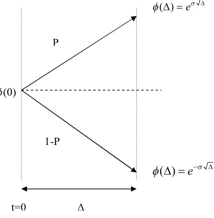
But how we can calculate the time horizon? Suppose,(), 0  is the output

price at time  and follows a geometric Brownian motion with drift parameter  and

volatility parameter  . Let  denote a small increment of time. Assume that current price of

output φ(0) is known. With the passage of  units of time the price of output either goes up

by the factor u with probability P or goes down by the factor d with the probability 1-P. As a

property of geometric Brownian motion model u, d and P are calculable and are equal to (see

Ross, 1999):



_e

u , _{d e} 

   



 _{ }



 

1 2 1

) 0 (



However, I will explain later that we need not have any knowledge about probability

distributions governing movements of prices in our analysis. The possible price movements

are shown in figure-2.

Figure 2 Probable steps of price in each period.

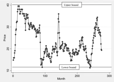
From the past we know how price has fluctuated over time. But given existing institutions

(e.g. market forces, laws, etc.), the extent of these fluctuations has never gone beyond an

upper and lower bound in a way such that  L where L is the difference between the two

bounds. This condition is indicated in figure-3.

We know that with current institutions, in each increment, price can shift with a

limited movement up or down. If for simplicity we suppose that 1, then price goes up to:

   

 t1  t e (1)

or comes down to:

 

 

 _{t1  t e} ₍₂₎ 



 

( ) e

σ√Δ

 







(

)

e

Δ P

1-P

Figure 3 Fluctuations of the price in the past.

10

20

30

40

P

ric

e

0 100 200 300

Month

Now suppose a carmaker wants to design and produce a car, and he does not know

where it will be driven. It can range from the highways of Germany to rough mountain roads

around the Himalayas. This carmaker never considers an average of these probable roads for

a proper design; instead, he tries to design a car, which can survive in the worst

circumstances. In the same way an entrepreneur in an uncertain environment, follows a best

worst strategy (he considers the worst movement of price and calculates whether under this

trend, the project can survive or not) instead of making a mathematical expectation of all

probable movements. Thus, he assumes for the purpose of designing the car the future price

to decrease by an amount given by Eq. (2). These price movements under the worst case

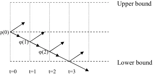
scenario are indicated in figure-4. Therefore, for instance, prices will attain 

 

 

and

 

 

t=0 t=1 t=2 t=3 φ(0)

φ(1)

φ(2)

happen thereafter? Under this assumption the price is compatible with profitability for t3

but not thereafter.

Figure 4 Steps of price in worst situations.

With the existing institutions, in the past prices have never become lower than the lower

bond. But there is no guarantee this time that price goes up after reaching the lower bound. It

might be the case that something has changed in the institutions that lets the price goes down

even more. We simply do not know what will happen next. This is the border between the

world of risks and uncertainties.

Consider a firm that produces one unit of merchandise in each period and there is no

variable cost. BL denotes the lower bound to price. Critical period, t*, is determined as

follows:

L t _B

e * 

) )( 0 (  

Therefore critical period t* _{will be:}

) ) 0 ( ln( 1

*

L

B

t 



 (3)

From (3) the critical period is decreasing in σ i.e. more unpredictability of the prices will lead

to the reduction in the time horizon within which the entrepreneur can rely on his information Upper bound

and forecasts. The entrepreneur calculates the discounted payback period for his project as follows: t t _r

I

d

e

t



_

_



)

(

where r is the discount rate and is considered constant by assumption. If the payback period t

calculated by Eq. (4) is greater than t*_{, then the project will be rejected. Projects with payback}

period equal or less than t* _{will be candidates for acceptance.}

For instance, consider a project with φ(0) = 100, σ = 0.3 I0 = 244, r =0.06 and lower

bound of price is BL = 30 and length of a period equal to a year. Assume that there is no

variable cost and one unit of output is produced each year. According to Eq. (3) we will have:

4 30 100 ln 3 . 0 1 * _       t

Then, we should calculate the discounted payback period for this project in the worst

circumstance. With respect to Eq. (4) we can calculate t as follow:



_e

_d



0 ) 06 . 0 3 . 0 (

₂₄₄

100



 ( 1) 244

36 . 0

100 0.36 _{ }

 _e t

 t=2.11

As t< t*_{, the project will qualify as a candidate for acceptance.}

If variance decreases along the time, which means we can have more precise

predictions of the future (maybe because of an improvement in institutions) then, the line of

price trends turn inside from 1 to 2 in figure-5. Because price will decrease more slowly than

before it reaches its critical level the critical time period for any given project will be higher

i.e. more investment can be incurred and more projects can be accepted.

(1)

(2) (3)

Upper bound 2

Upper bound 1

Lower bound 1 Lower bound 2 L2

L1 φ(0)

t=1 t=2 t=4 (1)

(2)

than before. As the critical period occurs sooner (say t = 1 in figure-5), there will be a

tendency to pick fewer projects – those with lower fixed costs and affording more liquidity

(e.g. non producing businesses like those of intermediaries which sometimes needs just a cell

phone as fixed cost). Therefore, not only the quantity but also the quality of investment

projects will change.

Figure 5 Changes in variance results in different critical periods.

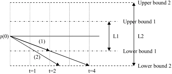
Assume fluctuations increase in a way that widen the range between upper and lower

bound (e.g. from L1 to L2 in figure-6). At first such fluctuations do not result in a revision of

the variance significantly. Therefore, the entrepreneur initially increases his investment and

accepts projects with a longer payback period (e.g. it changes from t = 2 to t = 4 in figure-6)

because he thinks that his projects would have more time to survive.

Figure 6 Effect of changes of fluctuations on upper and lower bounds.

Lower bound t=1 t=2 t=3 t=4 t=5

But, when these fluctuations gradually continue can increase variance and generate a wave of

pessimism among entrepreneurs, reducing their confidence in their predictions. The line of

price trends turns outside (e.g. from 1 to 2 in figure-6), reducing the critical period as well as

investments. As figure-6 shows the critical point with lower and upper bound 1 is reached in t

= 2. When the range shifts to L2 then critical period increases to t = 4 implying that

investment will increase. But the extent to which the critical period decreases after an

increase in σ will depend on the changes in L and σ. It could be greater or smaller than the

initial extent.

We can combine Eq. (3) and (4) with the interpretation that we will accept the

projects in which future discounted cash flows at least must be equal to the initial investment

in the critical time period. From Eq. (4) we will have:

)

(

t

I

d

e





_



As we assume that quantity of output is 1 in each period, therefore

)

(t

It

 is the rate of

investment at t and is denoted by ir thereafter. Solving the integral for τ will yield:

) 1

(

1 _{( r)t}*

r _r e

i _  



 

 (6)

Aggregating continuously over N individuals in each period of time, from Eq. (4) we

will have:

 





i

I

di

t

e

d

di

)

(

_



For simplicity we eliminate r.

Li i B t) ( 

is the value of current output deflated by the lowest level

of prices in the past. I denote it by yit and it can be supposed, for simplicity that yit , risks and

= y and φi(t) = φ(t). Therefore, the time horizon for each individual and for the entire

economy can be assumed to be a unique value t* 1_{. Thus, from Eq. (7) we have:}

 





i 0

I

di

t

e

d

di

)

(





_







( ) (1  )

* 0 t N i it e t N di I    



i it e

t N

di

I 

 _ 



The left hand side of Eq. (9) is the smallest ratio of aggregate investment to aggregate current

product and I denote it by IR . Thus, we have

 *

1 t

R e

I    (10)

Eq. (10) is very similar to Eq. (6) except that the cost of capital is eliminated. Substituting Eq.

(3) in (10) will yield



1

1_ 

 it

R

y

I (11)

where yit is

i i Lb t) ( 

as mentioned above. The rate of investment is a function of σ and yit. It

implies that higher ratios of output prices will increase the investment rate whereas increasing

uncertainty decreases the investment rate.

It can be shown that IR is non-increasing in σ for σ>0. From Eq. (11) we have

2 1 1       

I_R y_{it (12)}

Asyit 1, (12) is non-positive.

Figure 7 Increasing sigma reduces the rate of investment.

0

.2

.4

.6

.8

1

In

ve

st

m

en

t R

at

e

0 2 4 6 8 10

sigma

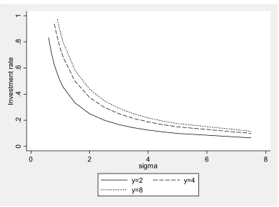
Figure 8 Higher level of price comparing to the lower bound increases investment rate.

0

.2

.4

.6

.8

1

In

ve

st

me

nt

ra

te

0 2 4 6 8

sigma

y=2 y=4

Figure-7 shows the IR for different extents of σ given y=4. Note that IR cannot become greater

than one because we cannot invest more than our income and it is a nonnegative amount. As

is clear in figure-7 the investment rate is decreasing in σ. Figure-8 indicates that a higher y

due to the a higher level of current price or reduction in lower bound (BL) will increases the

rate of investment at any given levels of uncertainty.

IV. Conclusion

In conclusion with the existing institutions in a country there would be a time horizon

within which investors could rely on their information and predictions. This time horizon

could be different from one country to another depending on institutions and institutional

changes over time. Increasing uncertainty will reduce this time horizon. This means that

investors will expect that current price might reach the lower bound sooner. Thus, they select

projects that can survive in the worst situations (i.e. continuously decreasing prices). Hence,

not only will investment decrease but its composition will also be biased toward the more

liquid projects.

Bibliography

Abel, Andrew B. and Janice C. Eberly, (1994), A Unified Model of Investment Under

Uncertainty, The American Economic Review 84(5),1369-1384.

Abel, Andrew B. and Janice C. Eberly, (1995), The effect of Irreversibility and Uncertainty

on Capital Accumulation., NBER working paper, No.5363, Advised 1998.

Abel, Andrew B. and Janice C. Eberly, (1996), Optimal Investment With Costly

Reversibility, The Review of Economic Studies 63(4), 581-593.

Abel, Andrew B, (1983), Optimal Investment Under Uncertainty, The American Economic

Arestis, Philip, (1996), Post-Keynesian economics: Towards Coherence, Cambridge Journal

of Economics 20,111-135.

Arrow, Kenneth J. ( 1968), Optimal Capital Policy with Irreversible Investment, In J.N.Wolfe

(ed.), Value, Capital and Growth. Papers in Honour of Sir John Hicks, Edinburgh:

Edinburgh University Press.

Bar-Ilan, Amer and William C. Strange, (1996), Investment Lags, The American Economic

Review 86(3), 610-622.

Craine, Roger, (1989), Risky Business the Allocation of Capital, Journal of Monetary

Economics 23, 201-218.

Davidson, Paul, (1991), Is Probability Theory Relevant for Uncertainty? A Keynesian

Perspective, The Journal of Economic Prespective 5(1),129-143.

Eisner, Robert and Robert H. Strotz, (1963), The Determinants of Business Investment, In

Englewood Cliffs. Commission on Money and Credit, Impacts of Monetary Policy. NJ:

Prentice Hall.S.

Hartman, Richard, (1972), The effects of Price and Cost Uncertainty on Investment, Journal

of Economic Theory 5,258-266.

Hartman, Richard, (1973), Adjustment costs, Price and Wage Uncertainty, and Investment,

The Review of Economic Studies 40(2),259-267.

Keynes, John Maynard, (1936), The General Theory of Employment, Interest and Money,

Great Britain: The Royal Economic Society.

Kregel, J.A. and Eric Nasica, (1999), Alternative Analyses of Uncertainty and Rationality:

Keynes and Modern Economics, In Premesse e Infuenze, S. Marzetti Dall, Aste

Brandolini and R. Scazzieri (eds.), La Probabilita in Keynes. Bologna: Clueb.

Kregel, J.A. (1983), Post- Keynesian Theory: An Overview, The Journal of Economic

Kregel, J.A. (1987), Rational Spirits and The Post Keynesian Macrotheory of Micro

Economics, de Economist 135(4),519-531.

Kregel, J.A. (1988), Irving Fisher, Great- Grandparent of the General Theory, Cahiers

d’Economie Politique 14-15, 59-68.

Kregel, J.A. (1998), Aspects of a Post Keynesian Theory of Finance, Journal of Post

Keynesian Economics 21(1),113-137.

Kregel, J.A. (1999), Instability, Volatility and Process of Capital Accumulation, in G.

Gandolfo and F. Marzano (eds.), Economic Theory and Social Justice. London:

Macmillan.

Leahy, John V. and Toni M. Whited. (1996), The Effect of Uncertainty on Investment: Some

Stylized Fact, Journal of Money, Credit and Banking 28(1), 64-83.

Modigliani, Franco and Merton H. Miller, (1958), The Cost of Capital, Corporation Finance

and the theory of Investment, The American Economic Review 48(3), 261-297.

Pindyck, Robert, (1991), Irreversibility, Uncertainty and Investment, Journal of Economic

Literature 29(3),1110-1148.

Pindyck, Robert, (1992), Investment of Uncertain Cost, NBER, Working Paper Series No.

4175.

Ross, Sheldon M. (1999), An Introduction to Mathematical Finance: Options and Other

Topics, Cambridge University Press.

Ross, Stephen A. and Randolph W. Westerfield and Bradford D. Jordan, (1998),