Munich Personal RePEc Archive
Forecasting macroeconomic variables
using a structural state space model
de Silva, Ashton
RMIT University
1 September 2008
Online at
https://mpra.ub.uni-muenchen.de/11060/
Forecasting macroeconomic variables using a structural
state space model
∗
Ashton de Silva
School of Economics, Finance and Marketing,
RMIT University
September 2008
Abstract
This paper has a twofold purpose; the first is to present a small macroeconomic
model in state space form, the second is to demonstrate that it produces accurate
forecasts. The first of these objectives is achieved by fitting two forms of a structural
state space macroeconomic model to Australian data. Both forms model short and
long run relationships. Forecasts from these models are subsequently compared to
a structural vector autoregressive specification. This comparison fulfills the second
objective demonstrating that the state space formulation produces more accurate
forecasts for a selection of macroeconomic variables.
keywords: State space, multivariate time series, macroeconomic model,
fore-cast, SVAR.
1
Introduction
The purpose of this paper is twofold; one, demonstrate how a state space model
may be formulated to capture the character of a structural vector auto-regressive
model, and two, show how this specification is useful for forecasting purposes. This
formulation will be referred to as astructural state space model.
Capturing economic relationships using a state space specification is not new.
Aoki & Havenner (1991) for instance model various US macroeconomic variables
including GNP and money stock. Another example is Balke & Wohar (2002) who
model low frequency movements of stock prices. A relatively recent example is
Pan-her (2007) who considers monetary and economic identities.
One key advantage of utilising the state space approach is that inter-series
rela-tionships can be disaggregated to the latent component level. This provides a greater
degree of insight which may be useful for policy analysis.
The structural state space model presented comprises two latent components for
each variable. They are referred to as the permanent and transitory component.
These components are specified such that they capture the long and short run
rela-tionships between variables. The specification is similar to the state space form of
the Beveridge-Nelson decomposition (Morley 2002).
The state space model described in this paper nests the structural vector
autore-gression (SVAR) specification. Eleven variables are used, six of which are classified
domestic as they can be considered to be within the sphere of influence of
Aus-tralian government authorities. The remainder of the variables represent the rest of
the world. As Australia is considered to be a small economy these variables are
considered to be determined “outside” the Australian economy.
The structure of this paper is as follows, a brief contextual outline is presented in
Section 2. In Section 3 the proposed state space approach is shown to be flexible
and simple to implement. The results of a forecast exercise are presented in Section
4. In Section 5 some concluding remarks are presented.
2
Background
The number of frameworks that have been employed to model relationships
be-tween macroeconomic variables are too numerous to mention. They include:
2007); and Dynamic Stochastic General Equilibrium (DSGE) specifications
(Mathe-son 2006). Arguably, the most popular in recent times (at least in the Australian and
New Zealand context) is the DSGE alternative. A technique that is also popular is
the Structural Vector Auto-Regressive (SVAR) framework (Berkelmans 2005, Buncic
& Melecky 2008, Fry et al. 2008).
As well as there being many frameworks, the size of these applications also vary
significantly, ranging from bivariate models (Moosa 1998) to large scale formulations
(Monash Model, Dixon & Rimmer 2002). A problem with large scale models is that
they can be particularly difficult to implement as they require the imposition of strong
economic assumptions that are often hard to verify1.
Although the class of macroeconomic models is large and diverse, any two
mod-els may be compared using the following two principles,degree of theoretical
coher-ence anddegree of empirical coherence. In every formulation a trade-off between
these two principles occur. For example: relative to the SVAR, the DSGE has more
theoretical coherence, whereas, the SVAR has more empirical coherence (Pagan
2003).
As the new formulation adopts the character of a SVAR approach it must also
share its qualities. That is, it has more empirical but less theoretical coherence than
the DSGE approach. However, as the structural state space formulation explicitly
models the permanent component, in this sense it may have more theoretical
coher-ence than the SVAR. Therefore, the framework presented might be considered to be
an improvement on the SVAR approach.
3
The State Space Model
The three key advantages2of the state space approach when compared to the (vec-tor) ARMA alternative are generality, flexibility, and transparency. For example, as
shown in this paper, it generalises easily to a multivariate formulation. The flexibility
of the framework is demonstrated by its ability to handle data irregularities such as
structural breaks. Finally, each series is decomposed into a set of latent components
that are directly estimated, thus illustrating the transparent nature of this approach.
The nature of these components is that they are determined before the model is fitted
1This problem is avoided in this paper as a small data set comprising only eleven variables has been
used.
2For an in depth discussion regarding the advantages of a state space approach refer to Durbin &
and are based on the stylised characteristics of the data. In addition, their contribution
may be gauged providing valuable insight into the underlying dynamics3.
The formulation adopted in this paper resembles the state space or unobservable
component form of the Beveridge-Nelson decomposition. This specification, in its
univariate form, has been employed in many instances. Perhaps the most notable
are Harvey & Jaeger (1993) and Proietti (2002). The multivariate form has also been
employed, applications include Morley (2002) and Sinclair (2005).
The link between the state space formulation presented in this paper and the
more common multivariate time series approaches has long been established
(Har-vey 1989, pages 431-432). It is important, however, to appreciate that analytical
equivalence does not automatically imply empirical equivalence (Hyndman 2001,
Morley et al. 2003).
The general specification for aN-variable system proposed is:
yt = µt+Wτt+ ΘXt+εt, εt∼N(0,Σε) (3.1)
µt+1 = δ+µt+Rµηt, ηt∼N(0,Ση) (3.2)
τt+1 = Φ(L)τt+Rτζt, ζt∼N(0,Σζ), (3.3)
whereyt,µtandτtdenoteN-vectors of observations, permanent components, and
temporary components at timet. Similarlyδis also anN-vector and represents a set
of constants. The termΦ(L)represents a polynomial function of the lag operatorL,
that isΦ(L) = Φ1L+ Φ2L2+. . .+ ΦpLpwhereLiyt=yt−i. TwoN×N coefficient
matrices are specified, ΦandW. TheΦ’s are estimated subject to the roots of the
polynomial function being larger than one, that is stationarity is imposed. The
distur-bances are assumed to be diagonal, independent and follow a Gaussian distribution.
They are denoted asεt,ζtandηt. The matricesRµandRτ are coefficient matrices
of dimensionN×N. For the remainder of this paperRτis constrained to be identity
matrix (IN). The termXtdenotes a set of exogenous variables at timet. The
coeffi-cient matrixΘmeasures the influences of the exogenous variables. In the context of
this paper,Xtcorresponds to a set ofqdummy variables.
The first equation, equation (3.1), represents the observation equation. It depicts
the vector of observations being comprised of two latent components, the
perma-nent and transitory compoperma-nent. The transitory compoperma-nent feeds into the observation
equation through the coefficient matrixW.
3As the aim of this paper is demonstrate the forecasting advantages of this specification the estimated
Equations (3.2) and (3.3) represent transition equations. The first of these is the
permanent component which is specified to be a random walk with drift. This may
also be referred to as the long run component. The second of these equations is
referred to as the transitory or short run component. The influence of this
compo-nent declines as the horizon increases. The temporary compocompo-nent is often referred
to as the cyclical component. The long run character of this specification may be
summarised as:
limT → ∞ yT =µ0+δ(T−2) +Rµ T−1
X
i=1
ηt−i+W T−1
X
i=1
Φ(L)ζT−i. (3.4)
Equation (3.4) shows that a set of observations at time T is determined by a
set of constantsµ0, deterministic linear trends (with growth rates), stochastic trends
PT−1
i=1 ηt−iand stochastic mean reverting processesPTi=1−1Φ(L)ζT−i.
3.1
Adopting a SVAR characterisation
In practice, before a SVAR can be fitted, the variables must be made stationary.
This is typically done by a series of transformations. In contrast, the structural state
space specification models the non-stationarity component explicitly in the form of a
permanent component equation.
By letting y˜t denote an N-vector of stationary observations at time t, for t =
1,2, . . . T, a SVAR(3) may be written as:
By˜t= Ψ1y˜t−1+ Ψ2y˜t−2+ Ψ3y˜t−3+et, et∼N(0,Σe) (3.5)
whereBandΨi(i= 1,2,3) denote coefficient matrices of dimensionN×N. In order
forB to be identifiable, there must be N(N2−1) restrictions imposed. Typically this is
achieved by constrainingBto be lower triangular. In addition, the covariance matrix
Σeis also constrained to be diagonal.
The transitory component of the structural state space model captures the
sta-tionary dynamics of a series and therefore may be formulated to adopt the character
of a SVAR specification. In particular, the characteristics of the SVAR specification
in the following way:
yt = µt+Wτt+ ΘXt+εt, εt∼N(0,Σε), (3.6)
µt+1 = δ+µt+Rηηt, ηt∼N(0,Ση), (3.7)
τt+1 = Φ1τt+ Φ2τt−1+ Φ3τt−2+ζt, ζt∼N(0,Σζ). (3.8)
The similarity between the SVAR model specified in equation (3.5) and the structural
state space model (equations (3.6) to (3.8)) is revealed by equatingτttoy˜t,W toB
andΦtoΨ. Arguably,τtcan be regarded as being a proxy fory˜t.
3.2
Two Macroeconomic Models of the Australian Economy
Both models proposed incorporate the characteristics of the SVAR model proposed
by Dungey & Pagan (2000). There was no particular reason for choosing the Dungey
& Pagan (2000) model except that it is the most well known Australian SVAR
specifi-cation. In general the characteristics ofanySVAR may be imposed on the framework
denoted by equations (3.6) to (3.8).
Two structural state space models are presented. The first treats the permanent
components as being independent. In contrast, the second allows the permanent
components to be related by estimating the off-diagonal elements ofRµ4.
The data set employed differs from Dungey & Pagan (2000) in that nominal
in-stead of real interest rates are used. The list of variables used are presented in Table
1.
OVERSEAS
USGDP
US real Gross Domestic Product
TOT
Terms of Trade
USR
90-day US Treasury Bill
USQ
US Q ratio
EXPT
Real Chain Weighted Exports
DOMESTIC
AUSQ
Australian Q ratio
GDP
Gross Domestic Product (Chained Volume Measure)
GNE
Real Gross National Expenditure
INF
Annual inflation rate
A3R
3-month Bank Bill
[image:7.595.164.481.116.179.2]RTWI
Real Trade Weighted Index
Table 1: Brief description of data set, see Appendix A for more details.
4For identification purposes the diagonal values ofR
Dungey & Pagan (2000) summarised the philosophy behind their model in three
points. First, Australia is a small open economy, therefore it cannot influence
over-seas markets. Second, a variable and all its lags would only be eliminated if it could
be justified. Third, some equations, like the inflation equation, reflect the findings of
single equation research. Having applied these three criteria, the restrictions applied
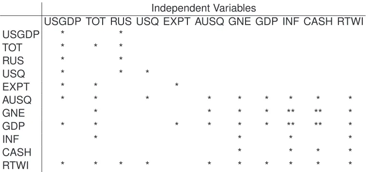
to the coefficient matricesW andΦare summarised in Tables 2 and 3.
Independent Variable
USGDP TOT RUS USQ EXPT AUSQ GNE GDP INF CASH RTWI
USGDP
1
TOT
*
1
RUS
*
1
USQ
*
*
1
EXPT
*
*
1
AUSQ
*
*
*
1
GNE
*
*
1
GDP
*
*
*
*
*
1
INF
*
*
1
CASH
*
*
1
[image:8.595.111.487.196.378.2]RTWI
*
*
*
*
*
*
*
*
*
1
Table 2: Contemporaneous Restrictions: * indicates a parameter is estimated, a value
of 1 is imposed for all diagonal elements and blank cells indicates no parameter is
esti-mated, i.e., restricted to zero
Independent Variables
USGDP TOT RUS USQ EXPT AUSQ GNE GDP INF CASH RTWI
USGDP
*
*
TOT
*
*
*
RUS
*
*
USQ
*
*
*
EXPT
*
*
*
AUSQ
*
*
*
*
*
*
*
*
*
GNE
*
*
*
*
**
**
*
GDP
*
*
*
*
*
*
**
**
*
INF
*
*
*
*
CASH
*
*
*
*
RTWI
*
*
*
*
*
*
*
*
*
*
Table 3: Restrictions on Autoregressive matrices, * denotes all lags of the variables are
present, ** denotes only the second and third lags are present. Blank cell indicates no
parameter is estimated, i.e., restricted to zero.
Enforcing these restrictions means that both state space models retain the key
characteristics of the SVAR outlined by Dungey & Pagan (2000). That is, the block
[image:8.595.110.492.455.633.2]the off-diagonals ofRµ introduces a new set of relationships, these are confined to
the permanent component. The two macroeconomic state space models applied take
the form previously stated exceptRζ =IN (see equations (3.6) and (3.8)).
The first and second models will be referred to hereafter as SSM1 and SSM2
(structural state space model one/two). SSM2 will model the basic form of long run
association between the eleven variables.
3.3
Estimation
Before the likelihood function is presented, the general form of equations (3.1) to (3.3)
is formally defined. These equations may be rewritten in the form of a two equation
system as:
yt = Ztαt+εt, εt∼N(0, H) (3.9)
αt+1 = Tαt+Rνt, νt∼N(0, Q). (3.10)
The models presented in the previous two sections are attained by setting:
Zt=
h
I B ON ON Xt
i
, αt=
µt τt
τt−1
τt−2
Θ T =
IN ON ON ON ON,q
ON Φ1 Φ2 Φ3 ON,q
ON IN ON ON ON,q
ON ON IN ON ON,q
ON ON ON ON Iq
, R=
Rτ ON ON ON ON,q
ON IN ON ON ON,q
ON IN ON ON ON,q
ON ON ON ON ON,q
Oq,N Oq,N Oq,N Oq,N Oq
νt=
whereIkandOkdenote the identity and null matrices of dimensionk×krespectively.
The terms0kandOi,jdenote ak-vector of zeros and a null matrix of dimensioni×j.
The estimation of this framework is straightforward. The likelihood to be
max-imised is
logL(Λ) =N T
2 log 2π− 1 2
T
X
t=1
log|Ft| − 1 2
T
X
t=1
νt′Ft−1νt′. (3.11)
The likelihood is calculated using the Kalman Filter. The prediction equations are
given by
at+1 = Tat|t, (3.12)
Pt+1 = T Pt|tT′+RQR′. (3.13)
The updating equations are
at|t = at+PtZ′Ft−1νt, (3.14)
Pt|t = Pt−PtZ′F1−1ZPt′, (3.15)
where
νt = yt−d−Zαt, (3.16)
Ft = ZPtZ′+H. (3.17)
Before the estimation procedure can be employed, a set of initial conditions need
to be determined. These initial conditions specify seed values for the states (α0 =
[µ0,τ0,τ0,τ0,Θ0]) and their variancesP0andQ0. Starting values for the coefficients
(W,Φ,δandR) also need to be determined.
Initial values for µ, τ and δ are determined simultaneously by running a linear
regression model. Specifically, the first ten observations of each variable (yi, i =
1, .., N) are regressed against a constant and a time trend. The initial value for the
permanent state is set to be the constant. Similarly, the estimated linear time trend
coefficient is used as the starting value forδ. Finally, the initial values of the temporary
state5are set to be the median of the residuals.
As the estimation process is initiated with a diffuse prior,P is set to be an identity
matrix with dimensions of4N+3, multiplied by a large number. Before this estimation
procedure is conducted however, the variances relating toΘare constrained to be
zero, thusΘis time invariant.
Two other second moment matrices need to be given starting values. These are
H and Q. The seed values forH correspond to the variance of each series. The
structure that is imposed onP is also imposed onQ. The firstN leading diagonals
are set to be the variance of each series. The following3Nleading diagonals are set
to be the variance of the first difference. Finally, the remaining three diagonals are
set to be zero.
According to Table 2, only a subset of elements are non-zero. These non-zero
elements are given a starting value of 0.8 as this was found to work well in practice.
EachΦwas set to be diagonal. The diagonal values were determined by fitting an
AR(3) to each variable.
As the exogenous variables are yet to be identified, the starting values forΘwill be
discussed briefly in the next section. The final set of coefficients that require starting
values are those in Rµ. As no prior information is available on what these values
might be, the matrix is initially set to be an identity matrix.
3.4
Specification of exogenous variables
The model is fitted to a data set of quarterly observations spanning 20 years. These
observations are non seasonal. The earliest observation corresponds to the first
quarter of 1985. Observations in years 2005 and 2006 are retained for an
out-of-sample forecast comparison. Plots of each variable is presented in appendix B.
Examination of the eleven variables suggests that three dummy variables is
ap-propriate. Each of these indicator variables relate to a specific domestic
macroe-conomic variable. The first is a double pulse dummy which is assigned to AUSQ.
This dummy variable captures the extraordinary growth observed in the second and
third quarters of 1987. The variable is given a value of 1 for these quarters and zero
elsewhere. The A3R variable exhibits a shift in the mean post 1992. Therefore the
variable is specified to be one pre-1992 and zero elsewhere. A similar story is also
evident for inflation. An inspection of the series reveals the Australian economy
ex-perienced considerably higher growth rates in the period 1985 to 1992, quarter 2. As
such, a dummy variable is specified to capture this phenomenon.
Having identified the exogenous variables, the starting values forΘcan now be
determined. In all three cases the linear trend equation that was outlined earlier is
the starting value forΘ.
4
Forecast comparison
The forecasting accuracy of the two structural state space models are compared by
conducting a roll-out forecasting comparison. As indicated in an earlier section the
observations corresponding to years 2005 and 2006 were withheld. These
obser-vations are now employed in a roll-out forecasting exercise. The maximum horizon
length is eight quarters.
The first batch of forecasts spans eight horizons and was generated by fitting the
SVAR, SSM1 and SSM2 to data ranging 1985 quarter 1 to 2004 quarter 4. The
second batch of forecasts spans seven horizons and was generated by fitting the
three alternatives to data ranging 1985 quarter 1 to 2005 quarter 16. This incremental
procedure was repeated eight times. The final prediction was a one step ahead
forecast corresponding to quarter 4 of 2006.
The measure used to compare the forecast accuracy is the mean absolute scaled
error (or MASE for short, Hyndman & Koehler 2006). This measure is chosen as
it is numerically robust, unlike conventional measures such as the mean absolute
percentage error (MAPE) and root mean square error (RMSE). Furthermore, the
measure is unitless and as such can be averaged across series. For anh-step head
forecast the MASE is:
MASE(h)= 1 |eT+h| T−1
PT
t=2|yt−yt−1|
As indicated above, the MASE is calculated by dividing the absolute forecast error by
the average of the absolute within sample first difference.
Three aspects of forecast accuracy will be examined. The first will consider the
accuracy across the entire data set. The second will focus on each variable
sepa-rately. The last will compare the approaches across horizons.
As part of the proceeding forecast evaluation formal hypothesis tests are
con-ducted. The test used is the Wilcoxen test. This test is a non-parametric test and
therefore is a function of order rather than magnitude. The motivation for using this
test is that at longer horizons the sample size is very small7.
6Before the models were fitted each variable was standardised by dividing through by its standard
devia-tion
4.1
Results
The relative forecasting accuracy of the state space models outlined earlier are
as-sessed in this section. The comparison begins by analysing overall forecasting
accu-racy.
Overall
Domestic Variables
Statistic
SVAR
SSM1
SSM2
SVAR
SSM1
SSM2
Min.
0.000
0.000
0.001
0.001
0.000
0.001
1st Qu.
0.013
0.030
0.020
0.016
0.016
0.013
Median
0.036
0.063
0.047
0.043
0.035
0.026
3rd Qu.
0.090
0.134
0.125
0.107
0.064
0.049
Max.
1.089
0.673
0.698
1.089
0.336
0.335
[image:13.595.143.452.169.283.2]Mean
0.090
0.109
0.097
0.134
0.056
0.045
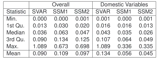
Table 4: Five Number Summary and Mean of Forecast Accuracy by Model
Table 4 displays a statistical summary of the overall forecasting accuracy for each
of the three approaches. By construction, all the scores are strictly non-negative. As
each raw score measures forecast error, a relatively smaller value is desirable.
The statistical measures used to summarise forecasting performance are the
min-imum,1st quartile, median, 3rd quartile, maximum and mean. Table 4 is separated
into two sections. The first is a general overview, the second considers a subset
corresponding to thedomesticvariables{AUSQ, GNE, GDP, INF, A3R, RTWI}.
For the domestic subset each statistic (excluding the minimum) indicates that the
state space models are noticeably more accurate. This is especially true for SSM2
where long run interrelationships are explicitly modeled. This conclusion is best
illus-trated by a comparison of the means, which show that the state space models have
inaccuracy measures less than half of that of the SVAR.
A similar analysis of the forecasting accuracy at the overall level does not indicate
the same conclusions, however the maximum values seem to indicate that the state
space models are more robust. Furthermore, as shown shortly, these results are
skewed by two poor performances and therefore not indicative of the true overall
performance. In addition, as the model is designed for an Australian context, it is the
variables which are within Australia’s sphere of control which are of primary focus. It
is thesedomesticvariables that the state space models are better at predicting.
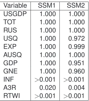
The second comparison examines forecasting accuracy on a variable by
vari-able basis. Positive values indicate that the state space models are more accurate.
Variable
SSM1
SSM2
USGDP
1.000
1.000
TOT
1.000
1.000
RUS
1.000
1.000
USQ
1.000
0.972
EXP
1.000
0.999
AUSQ
1.000
1.000
GDP
1.000
0.951
GNE
1.000
0.960
INF
>
0.001
>
0.001
A3R
0.020
0.004
[image:14.595.226.373.78.245.2]RTWI
>
0.001
>
0.001
Table 5: P-values relating to a one-sided Wilcoxon test for each variable, the test being:
H
0:
SSM
M ASE≥
SV AR
M ASEv
H
1:
SSM
M ASE< SV AR
M ASEperformed at least as well as the SVAR alternative. In particular, the state space
approaches performed noticeably better for the variables: USQ, EXPT, INF, A3R and
RTWI.
−0.4 −0.2 0.0 0.2 0.4
Forecast Accuracy by Overseas Variable
Variable
SVAR−SSM
−0.4 −0.2 0.0 0.2 0.4
USGDP TOT RUS USQ EXPT
SSM1 SSM2
−0.2 0.0 0.2 0.4 0.6 0.8
Forecast Accuracy by Domestic Variable
Variable
SVAR−SSM
−0.2 0.0 0.2 0.4 0.6 0.8
AUSQ GNE GDP INF A3R RTWI
[image:14.595.105.488.368.618.2]SSM1 SSM2
Figure 1: Forecast Comparison by Model.
Table 5 formally evaluates the differences between the state space models and
the SVAR alternative. The test employed was the Wilcoxon-test which is a
non-parametric test with the null corresponding to the case when the state space forecasts
are greater than or equal to the the SVAR alternative.
per-formed significantly better for three variables, inflation, Australian three month
trea-sury rate and real trade weighted index.
−0.4 −0.2 0.0 0.2 0.4 0.6 0.8
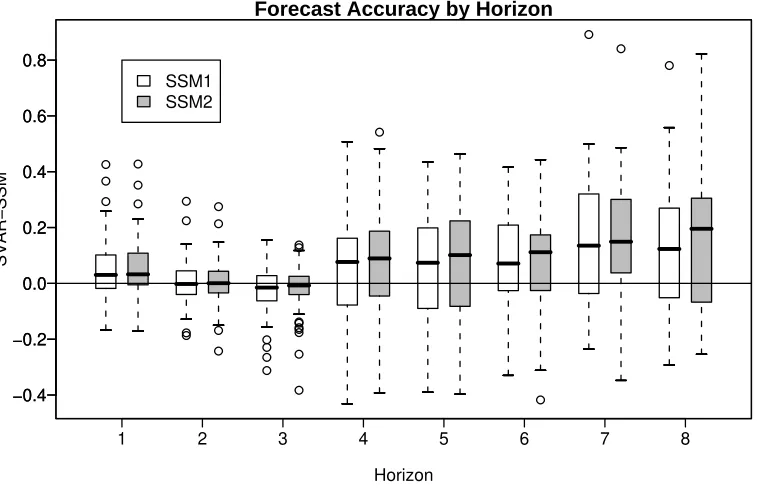
Forecast Accuracy by Horizon
Horizon
SVAR−SSM
−0.4 −0.2 0.0 0.2 0.4 0.6 0.8
1 2 3 4 5 6 7 8
[image:15.595.110.489.127.371.2]SSM1 SSM2
Figure 2: Forecast Comparison by Horizon (Domestic subset only).
Figure 2 displays the relative forecast accuracy for over horizons one to eight for
the domestic subset only. Careful examination of this figure suggests that as the
horizon increases the state space alternative becomes relatively more accurate. This
is especially true for the SSM2 which models the long run interrelationships.
Horizon
SSM1
SSM2
1
0.066
0.008
2
0.175
0.061
3
0.037
0.006
4
0.040
0.001
5
0.071
0.015
6
0.036
0.011
7
0.042
0.014
[image:15.595.232.365.497.621.2]8
0.094
0.031
Table 6: P-values relating to a one-sided Wilcoxon test for each horizon (domestic subset
only), the test being:
H
0:
SSM
M ASE≥
SV AR
M ASEv
H
1:
SSM
M ASE< SV AR
M ASEUsing the Wilcoxon-test to verify the pattern observed in the box and whisker plots
confirms the better performance of the state space approach. According to Table 6,
at the 10% significance level only once can the null not be rejected. That is, across all
the state space alternative are superior.
5
Conclusion
The purpose of writing this paper was twofold, one to illustrate how the state space
approach can be formed to represent a small open macroeconomic model and two,
demonstrate that forecasts from this adaption are accurate. On both accounts this
paper has satisfied these objectives.
In particular, the first objective was achieved (in part) by showing how the
charac-ter of a SVAR specification may be incorporated into a structural state space model.
Furthermore, long run (inter) relationships were explicitly modeled and showed to
have a positive effect on forecast accuracy at longer horizons. Also, the advantages
of the state space model were presented, these being generality, flexibility and
trans-parency.
Improvements in forecast accuracy have also been demonstrated. This was
par-ticularly true for the domestic subset. In general the Box and Whisker plots of the
previous section demonstrate that the structural state space model performed at least
as good as the SVAR on eight occasions.
In summary, the evidence provided suggests that the structural state space
ap-proach is a useful forecasting tool that can yield significant improvements when
com-pared to a standard alternative.
References
Aoki, M. & Havenner, A. (1991), ‘State space modeling of multiple time series’,
Econometric Reviews10, 1–59.
Balke, N. S. & Wohar, M. E. (2002), ‘Low-frequency movements in stock prices: a
state-space decomposition’,The Review of Economics and Statistics84(4), 649–
667.
Berkelmans, L. (2005), Credit and monetary policy: An australian SVAR, Technical
report, Reserve Bank of Australia.
Buncic, D. & Melecky, M. (2008), ‘An estimated new keynesian policy model for
Diebold, F. X. & Mariano, R. S. (1995), ‘Comparing Predictive Accuracy’,Journal of
Business and Economic Statistics5, 253–263.
Dixon, P., Parmenter, B., Sutton, J. & Vincent, D. (1997), ORANI: A Multisectoral
Model of the Australian Economy, North Holland.
Dixon, P. & Rimmer, M. (2002),Dynamic General Equilibriun Modelling For
Forecast-ing And Policy, North Holland.
Dungey, M. & Pagan, A. (2000), ‘A structural VAR of the Australian economy’,The
Economic Record76, 321–342.
Durbin, J. & Koopman, S. (2001), Time Series Analysis by State Space Method,
Oxford.
Fry, R., Hocking, J. & Martin, V. (2008), ‘The role of portfolio shoocks in a
struc-tural autoregressive model of the australian economy’, The Economic Record
84(264), 17–33.
Harvey, A. C. (1989),Forecasting, structural time series models and the Kalman filter,
Cambridge University Press, Cambridge.
Harvey, A. & Jaeger, A. (1993), ‘Detrending, stylised facts and the business cycle’,
Journal of Applied Econometrics8, 231–247.
Hyndman, R. J. (2001), ‘It’s time to move from ’what’ to ’why”,International Journal
of Forecasting17, 567–570.
Hyndman, R. & Koehler, A. B. (2006), ‘Another look at measures of forecast
accu-racy’,International Journal of Forecasting22, 679–688.
Matheson, T. (2006), Assessing the fit of small open economy dsges, Technical
re-port, Reserve Bank of New Zealand.
Moosa, I. (1998), ‘An investigation into the cyclical behaviour of output, money, stock
prices and interest rates’,Applied Economic Letters5, 235–238.
Morley, J. C. (2002), ‘A state-space approach to calculating the Beveridge-Nelson
decomposition’,Economics Letters75, 123–127.
Morley, J. C., Nelson, C. R. & Zivot, E. (2003), ‘Why are the Beveridge-Nelson and
unobserved-components decompositions of GDP so different?’, The Review of
Nimark, K. (2007), A structural model of australia as a small open economy, Technical
report, Reserve Bank of Australia.
Pagan, A. (2003), An examination of some tools for macro-econometric model
build-ing,in‘METU Lecture at ERC Conference VII, Ankara’.
Panher, G. S. (2007), ‘Modelling and controlling monetary and economic identities
with constrained state space models’,International Statistical Reveiw75, 150–169.
Proietti, T. (2002), Some reflections on trend-cycle decompositions with correlated
components, Working Paper, Department of Economics, European University
In-stitute.
Sinclair, T. (2005), Permanent and transitory movements in output and
unemploy-ment: Okun’s law persists, Working Paper, Department of Economics, Washington
University.
A
Description of Data used
USGDP Real Gross Domestic Product of USA. Data Source: Bureau of Economic
Analysis{http://www.bea.gov/}, issue date 20/12/2007.
TOT Terms of Trade (AUS). Data Source: Australian Bureau of Statistics, Catalogue
5206, Table 1.
USR 3 month US Treasury Bill. Data Source: Federal Reserve. Identifier: H15/H15/RIFSGFSM03 N.M.
This series was calculated by averaging the monthly observations for each
quar-ter.
USQ US Q ratio. Calculated by averaging the monthly S&P500 index and then
di-viding it by the USA Implicit Price Deflator. The IPD was downloaded from the
Bureau of Economic Analysis.
EXPT Real exports of Goods and Services. Source: Datastream, Code: AUOCFEGSD.
AUSQ Australian Q ratio, calculated in the same way as USQ. Date Source:
Austal-ian Bureau of Statistics (ASX200) and Reserve Bank of Australia (IPD).
GDP Chain Weighted Volume Gross Domestic Product of Australia. Source ABS,
Table 5206.0.
GNE Australian Gross National Expenditure. Source: Datastream
A3R 3-month Bank Bill. Average of monthly observations. Source: RBA
B
Plots of the Data
USGDP
1985 1990 1995 2000 2005 4.0 4.5 5.0 5.5 6.0 6.5 7.0 TOT
1985 1990 1995 2000 2005 7 8 9 10 11 USR
1985 1990 1995 2000 2005 1
2 3 4
USQ
1985 1990 1995 2000 2005 1.0 1.5 2.0 2.5 3.0 3.5 4.0 EXPT
[image:20.595.113.493.103.369.2]1985 1990 1995 2000 2005 1.5 2.0 2.5 3.0 3.5 4.0
Figure 3: Plots of overseas.
AUSQ
1985 1990 1995 2000 2005 2 3 4 5 6 AUSGDP
1985 1990 1995 2000 2005 3.5 4.0 4.5 5.0 5.5 6.0 6.5 GNE
1985 1990 1995 2000 2005 3.0 3.5 4.0 4.5 5.0 5.5 6.0 INF
1985 1990 1995 2000 2005 0
1 2 3
A3R
1985 1990 1995 2000 2005 1.0 1.5 2.0 2.5 3.0 3.5 4.0 RTWI
1985 1990 1995 2000 2005 9.5 10.0 10.5 11.0 11.5 12.0 12.5
[image:20.595.110.494.206.634.2]