Unequally spaced knot techniques for the numerical solution of partial differential equations

Unequally spaced knot techniques for the numerical

solution of partial differential equations.

WISHER, Stephen J.

Available from Sheffield Hallam University Research Archive (SHURA) at:

http://shura.shu.ac.uk/20555/

This document is the author deposited version. You are advised to consult the

publisher's version if you wish to cite from it.

Published version

WISHER, Stephen J. (1983). Unequally spaced knot techniques for the numerical

solution of partial differential equations. Doctoral, Sheffield Hallam University (United

Kingdom)..

Copyright and re-use policy

See http://shura.shu.ac.uk/information.html

Sheffield Hallam University Research Archive

Z Q 4 - 5 B 3 2 0 J»Z

Sheffield City Polytechnic Library

REFERENCE ONLY

ProQuest Number: 10701202

All rights reserved

INFORMATION TO ALL USERS

The quality of this reproduction is dependent upon the quality of the copy submitted.

In the unlikely event that the author did not send a com plete manuscript and there are missing pages, these will be noted. Also, if material had to be removed,

a note will indicate the deletion.

uest

ProQuest 10701202

Published by ProQuest LLC(2017). Copyright of the Dissertation is held by the Author.

All rights reserved.

This work is protected against unauthorized copying under Title 17, United States C ode Microform Edition © ProQuest LLC.

ProQuest LLC.

789 East Eisenhower Parkway P.O. Box 1346

UNEQUALLY SPACED KNOT TECHNIQUES FOR THE

NUMERICAL SOLUTION OF PARTIAL DIFFERENTIAL EQUATIONS

Being a thesis submitted

in partial fulfilment of the degree of

Doctor of Philosophy

at

Sheffield City Polytechnic

by

STEPHEN JOHN Y/ISHER

ACKNOWLEDGEMENTS

I wish to express my sincere thanks to my Director of

Studies, Dr G F Raggett, for his general support,

constructive criticism and continual encouragement during

my work on this thesis.

I would also like to thank numerous members of the Department

of Mathematics, Statistics and Operational Research at

Sheffield City Polytechnic for many helpful discussions;

particular thanks are due to Dr A C Allen, Dr R McLaughlin,

Mr R Ward and, my second supervisor, Dr J A R Stone.

I wish to acknowledge a very helpful discussion which took

place between myself, Dr Raggett and certain members of

the Division of Numerical Analysis and Computer Science at

the National Physical Laboratory. Particularly, I wish to

thank Dr M G Cox for bringing to my attention the variable

knot point results for approximation on which two of the

methods of this thesis are based.

My thanks are also due to Mrs Renee Hayes for her expert

typing of this thesis.

ABSTRACT OF THE THESIS

"Unequally Spaced Knot Techniques for the Numerical

Solution of Partial Differential Equations"

S J WISHER

Cubic spline approximations to time dependent

partial differential equations, having both constant and variable coefficients, are developed in which the knot points may be chosen to be unequally spaced. Four methods are presented for obtaining 'optimal* knot positions, these being chosen so at to produce

an increase in accuracy compared with methods based on equally spaced knots. Three of the procedures described produce knot partitions which are fixed throughout time. The fourth procedure yields

differently placed 'optimal' knots on each time line, thus enabling us to better approximate the varying time nature characteristic of many partial

differential equations. Truncation errors and stability criteria are derived and full numerical implementation procedures are given. Five case studies are presented to enable comparisons to be drawn between the knot placement methods and results found using equally spaced knots. Possible extensions of the work of this thesis are given.

CONTENTS

Page No,

Acknowledgements

Abstract of the thesis

Chapter 1 Introduction

1.1 Finite Difference Solution of Partial Differential Equations

1.2 Development of Spline Techniques

1.3 Motivation for Present Work

i

ii

Chapter 2 Review of Cubic Spline Theory

2.1 Definition of a Cubic Spline

2.2 Cubic Spline Functions

10 10

Chapter 3 Initial Value Partial Differential Equations with Equally Spaced Knots

(i) Hyperbolic Partial Differential Equations

3.1 Constant Coefficients

3.2 Variable Coefficients

(ii) Parabolic Partial Differential Equations

3.3 Constant Coefficients

3.4 Variable Coefficients

14

19

21

29

Chapter 4 Initial Value Partial Differential Equations with Unequally Spaced Knots

Page No.

4.2

4.3

Chapter 5

Hyperbolic Partial Differential Equations with Constant Coefficients

Parabolic Partial Differential Equations with Constant Coefficients

Methods for Obtaining Knot Partitions

35

43

5.1 Preamble 47

5.2 A Local Method 48

5.3 A Global Method 52

5.4 A Transformation Method 58

Chapter 6 Case Studies 1

6 . 1 Case Study Philosophy 62

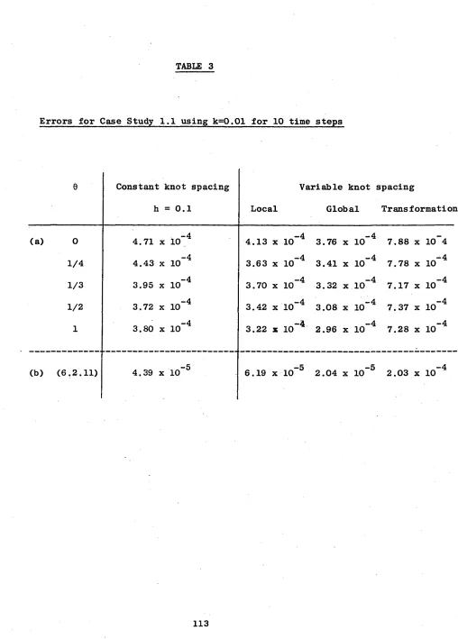
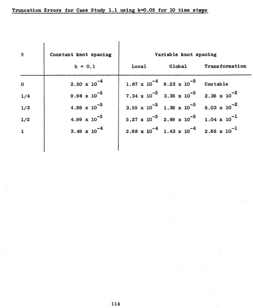
6 . 2 Case Study 1.1 62

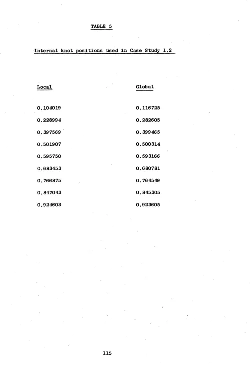
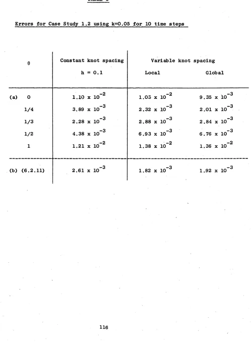
6.3 Case Study 1.2 69

6.4 Case Study 1.3 72

6.5 Case Study 1.4 74

6 . 6 Case Study 1.5 77

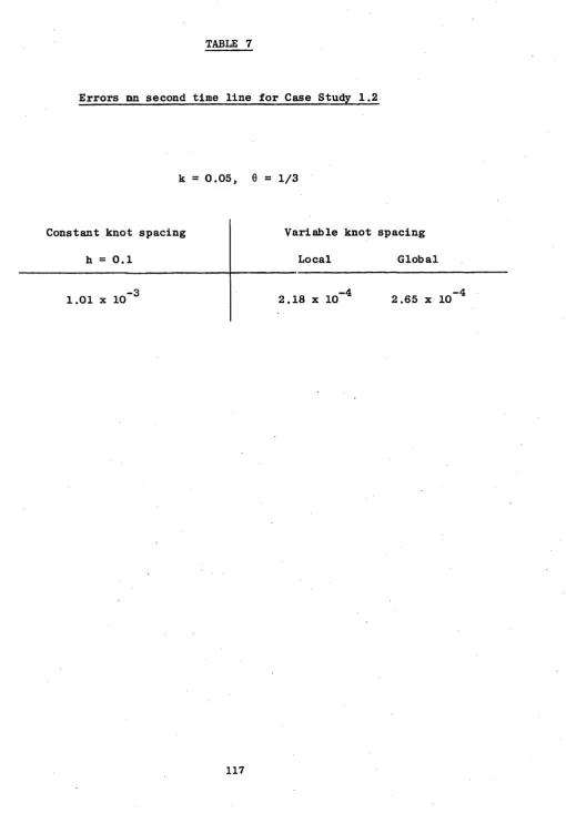
Chapter 7 Varying the Knots on Each Time Line

7.1 Preamble 82

7.2 Procedure for Determining Optimal

Knot Partition 83

7.3 Implementation of the Splines Scheme 87

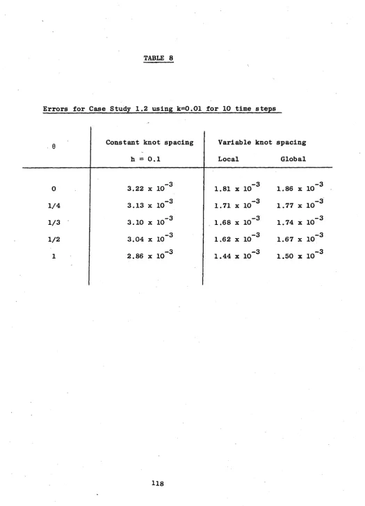
Chapter 8 Case Studies 2

8 . 1 Case Study Philosophy 89

8 . 2 Case Study 2.1 90

Page No.

8.4 Case Study 2.3 94

8.5 Case STudy 2.4 96

8 . 6 Case Study 2.5 97

Chapter 9 Conclusions and Extensions

9.1 Conclusions 1 0 1

9.2 Possible Extensions 108

Tables 111

Figures 142

Appendices 165

CHAPTER 1

. Introduction

1.1 Finite Difference Solution of Partial Differential Equations

The most well-known early work on the use of finite

differences was that of Richardson (1910), although the

paper by Courant, Friedrichs and Lewy (1928) is usually

considered as the birthplace of modern numerical methods

for solving partial differential equations. In that work

Courant, Friedrichs and Lewy also showed that the

convergence of simple difference approximations depends

on the mesh ratio satisfying certain conditions. Such

conditions were also derived using Fourier techniques for

a wide variety of problems by von Neumann during the

Second World War. A detailed discussion of von Neumann's

work is given in O'Brien, Hyman and Kaplan (1951).

Since the work of von Neumann many finite difference schemes

have been proposed, perhaps the most well-known being that of

Crank and Nicolson (1947). A thorough description of methods

available is given in Richtmyer and Morton (1967). The

computational aspects and the application of finite

difference methods to partial differential equations with

variable coefficients and generalised boundary conditions

is discussed in, for example, Ames (1977), Mitchell (1969)

and Mitchell and Griffiths (1980).

The majority of finite difference schemes derived for

the solution of time dependent partial differential

equations use rectangular grids which have constant

step lengths in both the space and time directions.

There are} however, certain instances in which unequally

spaced mesh points in the space direction are beneficial.

For example, situations frequently arise in which the

solution of a partial differential equation varies very

rapidly over a small part of the domain but changes slowly

over the rest of the domain. The problem in using non-

uniform grids in such situations is that, in general, an

order of accuracy is lost by employing unequally spaced

mesh point schemes. It is therefore important to position

the mesh points so that optimal numerical performance is

achieved. Pearson (1968) proposed an iterative scheme for

the solution of boundary layer problems in which additional

mesh points are added where the variation in solution values

exceeds some predetermined level. Woodford (1975) extended

this idea and produced a scheme which used graded meshes

in which the mesh points are systematically chosen according

to the natural structure of the problem. The use of such

transformation techniques has also been considered by

various authors (see, for example, Jones and Thompson (1980)

and references therein) in determining the position of mesh

points for the solution of fluid flow problems.

An additional area where non-uniform grids have been

used is in the numerical solution of moving boundary

problems in heat flow* Murray and Landis (1959) solved

such so-called Stefan problems by employing a uniform grid

on the solid side of the boundary and a different uniform

grid on the liquid side. A change in the size of the step

lengths therefore occurs from one side of the boundary to

the other. These moving boundary problems were also

considered by Douglas and Gallie (1955). They used a

scheme with a variable time step length which is chosen so

that the boundary always moves from one line of the space

grid to the neighbouring line in a single time step. More

recently, Crank and Gupta (1972b),proposed a method for

solving Stefan problems which employed cubic splines to

interpolate solution values.

Development of Spline Techniques

The term ’spline function’ was first used by Schoenberg

(1946) in a paper describing the use of generalised splines

and other piecewise polynomials to approximate smooth

functions of one variable. Although Schoenberg’s early

paper was an important contribution to the use of spline

techniques, it was not until the 1960's that further work

in the field was published.

Since that time, spline functions have been used

extensively as methods of interpolation and approximation,

see for example, Birkhoff and de Boor (1967), Greville (1969),

Schumaker (1969), Curtis (1970), Hayes and Halliday (1974)

and Cox (1975). An excellent summary of spline techniques

is given in Ahlberg, Nilson and Walsh (1967).

Due to the benefit gained by employing splines in approximation

problems, numerous authors have adapted spline techniques to

obtain solutions to various problems in numerical analysis.

For example, Loscalzo and Talbot (1967), Loscalzo (1969),

Micula (1973) and Patricio (1978) considered the solution

of initial value problems, whilst methods for solving

two-point boundary value problems were presented by Bickley

(1968), Albasiny and Hoskins (1969) , Fyfe (1969) and

Khalifa and Eilbeck (1982).

in addition, El Tom (1974 and 1976) has used spline techniques

in the solution of Volterra integral equations.

The development of spline techniques for obtaining numerical

solutions to partial differential equations began with

Papamichael and Whiteman (1973) . In that work the authors

presented a method for solving the simple one-dimensional

spline approximation in the space direction together with

a finite difference approximation in the time direction.

A similar technique was used by Raggett and Wilson (1974)

in obtaining numerical solutions to the one-dimensional

wave equation.

Spline function approximations have since been applied

to more general partial differential equations. For example,

Raggett, Stone and Wisher (1976) considered the solution

of practical problems modelled by hyperbolic partial

differential equations of the form

a(x,t) jhi + b(x,t) jhi + c(x,t)u. (1 .2 .1)

8x _ 8x

In addition, Rubin and Graves (1975) and Rubin and Khosla

(1976) presented spline techniques for solving problems in

fluid mechanics. In particular, their work developed the

use of spline techniques in the solution of non-linear

equations. The application of spline function approximations

to partial differential equations in two space dimensions

was considered by Jain and Holla (1978) . They proposed a

high accuracy formula, using a technique similar to that

of McKee (1973) , for the spline solution of wave equations of

a

8t^ 3x

the form

92u = a(x,y,t) 32u + b(x,y,t) 32u . (1 .2 .2 )

8t2 9x2 3y2

Jain and Aziz (1981) have also recently applied parametric

spline techniques to a variety of differential equations and

have found that they compare favourably with the more usual

cubic spline approximations. In addition, papers by Sastry

(1976) and Pala and Spano (1978) have also proposed methods

for obtaining spline solutions to parabolic partial

differential equations.

1.3 Motivation for Present Work

As mentioned earlier, the use of cubic splines for the

numerical solution of the one-dimensional wave equation

has been considered by Raggett and Wilson (1974). An

indication of how that work could be generalised to the

solution of more general one-dimensional, constant coefficient,

hyperbolic partial differential equations was shown by

Raggett (1974). The completion of that work was carried

out by Wisher (1977) , who indicated that the use of spline

techniques gave increased accuracy over comparative

hyperbolic equations by Wisher (1977) are illustrated in

Chapter 3 of this thesis. The extension of that work to

include parabolic partial differential equations is also

given in Chapter 3.

Most of the previously mentioned works on the application

of spline techniques to the solution of partial differential

equations have produced methods in which the knots were

chosen to be equally spaced. An exception here is that of

Wisher (1977) who used unequally spaced knots in solving

the simple wave equation. In that work, the knots were

positioned in an ad-hoc manner and no improvement in

accuracy was observed over the use of uniform knot partitions.

Further, some experimentation on choosing the knot points

to be the zeros or extrema of the shifted Chebyshev polynomial

T*(x) = Cos (nCos-1 (2x-l)) (1.2.3)

n

was undertaken in Wisher (1977). Again no improvement in

accuracy over constant knot spacing was observed.

In this thesis we employ spline techniques with unequally

spaced knots for the numerical solution of both hyperbolic

and parabolic partial differential equations. Further, we

present methods for the optimal positioning of these knots.

The derivation of schemes allowing the non-uniform partitioning

of knot points is given in Chapter 4.

The problem of determining optimal positions of knots

has been shown to be a difficult one and has only to-date

been applied to approximation problems.

In the earlier works on approximating functions (see for

example, Curtis and Powell (1967)) equally spaced knots

were employed with additional knots being inserted when -

the error in the approximation was larger than some

prescribed magnitude. Since that time various authors

have attempted to choose the positions of the knots, in

some optimal sense, given knowledge about the function f

being approximated. De Boor and Rice (1968) described an

algorithm for solving the least-squares cubic spline

approximation problem. Their idea was to vary one knot

at a time so as to reduce the error of best approximation.

Similarly, Esch and Eastman (1969) proposed a method for

a best discrete Chebyshev approximation by splines. Both

these algorithms are computationally expensive and de Boor

(1973) has since proposed an alternative method which chooses

the knot partition from the given function f. This method

in Chapter 5 by taking the function f to be the given

initial condition. Two additional methods for optimally

positioning the knots are also derived in Chapter 5.

In Chapter 6 of this thesis, a number of case studies

are considered and solutions derived using knot partitions

resulting from each of the methods given in Chapter 5.

Comparisons are also made with results produced using equally

spaced knots.

The results of Chapter 6 suggest that improvement on the

methods for locating the knot points given in Chapter 5 would

be desirable. An improved algorithm is thus presented in

Chapter 7, which chooses optimal partitions of knots on each

time line. The suitability of this method is examined in

Chapter 8 , where the earlier case studies are again considered.

Throughout this thesis, no particular reference to the

associated characteristics has been made for hyperbolic

problems. However, it should be realised that due

account has been taken in the satisfaction of the

Courant Friedrichs Lewy condition (see Mitchell and

Griffiths (1980)) for all the problems cited.

CHAPTER 2

Review of Cubic Spline Theory

Definition of a Cubic Spline

Let f(x) be a function with continuous derivatives in

the range a $ x $ b. To approximate f(x) using cubic

spline techniques we may subdivide the interval a $ x $ b

into N sub-intervals by inserting knots x^ such that

a = Xq < x^ < ....< xN = b. (2.1.1)

S(x) is a cubic spline interpolating to the function f(x) at

the knots x^, x if

(i) in each sub-interval x^^ $ x $ x^^ (1=1,2, ... ,N) f

S(x) is a cubic polynomial,

(ii) s ’(x) and s"(x) are continuous everywhere in [a ,bJ ,

(iii) S(x±) = fCxJ (i=0,l,...,N).

A cubic spline thus consists of a set of cubic polynomial

arcs which are joined smoothly end to end with continuous

first and second derivatives. In general, the third derivative

will have a discontinuity at each of the knots x ,x ,....,x^ - ^

Cubic Spline Functions

where hi = Xi Xi l Ci = 1,2,...,N) (2.2.2)

ft

and = S (x_^) . Integrating twice gives the cubic spline function S(x) on I x, , x I as

S(x) = (x± - x)3 + M± (x - Xj.j)3 +/ “ h)2 ) (*,“*)

6h± 6h± \ 6 ' hi

+ | f(Xi) - h± 2 M± | (x - xi ]L) (i=l,2,----,N)

(2.2.3)

the constants of integration being evaluated from S(x^) = f(x^)

and S(x^, ^) = f(x^ ^) . From (2.2^3) the following one-sided

limits of the derivatives of s'(x) are derived

s'(Xi-) = h± U ±mml + h ± Mi + f(x±) - f(xi-_1) (i=l,2,...,N)

6 3 hi (2.2.4)

S ’(x±+) = -hi + 1 M± - hi + 1 Mi + 1 + f(x±+1) - f(x±) (i=0,l,...(N-l))

3 6 hi+l (2.2.5)

The unknowns M (i=0,2,...,N) are obtained by equating these

one-sided limits, thus giving

h. M , + h.+h. _{l i} M. + h. M. = h.f(x. .J-Oi.+h, ,)f(x.)+h, \ f(x. .

- 1 l l+l i i+ 1 i+ 1 i i+ 1 i i+ 1 l i+ 1 i-l

6 3 6 h.h. ,

l l+l

(i=l,2,...,(N-l))

(

.

.

)

Equation (2.2.6) is a tri-diagonal system of (N-l)

equations in (N+l) unknowns. To solve this system various

choices of conditions are available at the end points,

Xq and x^, of the interval to produce a consistent set

of (N+l) equations

(i) s"(x^) = 0 (i=0,N) (2.2.7)

(ii) S * (x^) ■= f*(xi) (i=0,N) (2.2.8)

(III) s " ^ ) = f’* (x±) (i=0,N) (2.2.9)

As suggested by Behforooz and Papamichael (1979), the

choice of these extra conditions plays an important role

on the quality of the spline approximation. It is well-known

that the best order of approximation which can be achieved

by an interpolatory cubic spline is

I[ S - f 11 = 0(h4)

where | | . | | denotes the uniform norm on [a>bJ aad

h = max(h^). This order of accuracy is obtained if either

(ii) or (iii) are used as the extra conditions. As stated 4

by Kershaw (1973) an 0(h ) accuracy is not obtained if

condition (i) is applied. However, the conditions (ii)

and (iii) require knowledge of the derivatives of the

function f(x). This knowledge is not generally available

from any imposed boundary conditions of partial differential

this thesis, S(x) and (i) being known as a ’natural’

cubic spline. Papamichael and Worsey (1981) have

recently derived improved extra conditions for spline

approximation which could result in increased accuracy

to the results of case studies considered later.

Having decided on the choice of 'end conditions', substitution

of these into (2.2.6) gives a system of (N-l) equations which

are linearly independent, tri-diagonal and diagonally

dominant. They can therefore easily be solved for M.i

(1=1,2,...,(N-l)), the satisfaction of the end conditions

then giving MQ and The spline function S(x) can then

be obtained from (2.2.3).

CHAPTER 3

Initial Value Partial Differential Equations with Equally Spaced Knots.

(i) Hyperbolic Partial Differential Equations

3.1 Constants Coefficients

Suppose that u(x,t) satisfies the second order linear

hyperbolic partial differential equation

2 2

8 u = a 8 u + b jhi + cu (0 £ x $ 1, t >0) (3.1.1)

2 2

8t 8x dx

where the coefficients a, b, c are constants (a > 0 ).

Assume further that (3.1.1) is subject to the function

value boundary conditions

u(0,t) = f1 (t) , u(l,t) = f2 (t) (3.1.2)

and the initial conditions

u(x,0) = g (x) , 8u(x,0) - g (x) (3.1.3)

8t

where f^(t), fg(t), g^x) and g2 Cx) are known functions.

To obtain solutions to (3.1.1) using spline techniques

we here consider the knots

0 . = x < x < .... < xXT = 1 _{0 1 N} (3.1.4)

to be.equally spaced where the distance between successive

knots is h, so that xi = ih (i=0,l.... ,N) . We now replace

the time derivative in (3.1.1) by a finite difference

approximation and the space derivatives by a cubic spline,

thus obtaining at the point (ih,jk) the implicit relationship

u. . ,-2u. ,+u. . _ = afsM. . _+(l-20)M. J+0MJ ._{i,d i,j+l I i,j-l i,j i , j+lj}

+ M 0l, .. _ +(1-2 0)L +0L L

\ i,j-l i , d i,d+lj

+ c(0u. +(1-2 0)u +0u \

I (3.1.5)

(i=0,l,....,N; d=l»2 ,»**»; ; 6 ^ 0)

where L = S*(x ), M = s"(x ); S (x) denoting the

1 13 J * J J ^ J

th cubic spline interpolating the values u on the d

1 »J

time line, this being given by

Y x ) " (v x ) 3 + Mi.,i(x-xi-i) 3 + f ui-i..r^Mi-i..i) (xr x)

6h 6h \ / h

* y * t j_-2"i j

j

As shown in section 2.2, the continuity of the first

derivatives of the spline function yields

i J + 2 M J . = u. , . - 2uJ , + u, , .

k i-1,3 o' i»d fi- i+1,3 i-1,3 i.d i+1.3

2 (3.1.7)

h

(i=l,2,....,(N-l))

th th

This relationship also holds on the (d-1) and (d+1)

time lines, giving respectively

i Mi-l,j-l+ |Mi,j-l+ = Ul-1 . j-l~2Ui ..1-l'l'Ul+l. j- 1

h2

(1=1,2...,(N-1)) (3.1.8) and

iMl-l, j+l + |M1 , j+ 1 + £“i+l, j+l = Ul-1 . ,1+l~2Ui . ,1+1+U1+1 . j+ 1

h2

(1=1,2...(N-l)) (3.1.9)

We now require an expression similar to (3.1.7) which th

incorporates the L _{1 , J} values. On the j time line (2.2.4)and (2.2.5) respectively become

L_, a = S J(xJ-) = hM , u + hM + u_, - u^

h--- <3

J - o v * - n m - . T U ffl - r u - u

i,j

j i

ij

i

j

i-l>

(3

(3 (i=l,2.... ,N)

and

L. = S*(x. +) = -hM. -hM. + u ' • u. .

i j j i 3 g 1 +1,J i+l,J - i.d

(1=0,1,--- ,(N-1)) From (3.1.10) we have

It, , . = hMJ . + hM. , . + ^ , . — u. .

i+l,j J i+l.J i+l.j i,j

h

<i=0> 1,--- - (N-l))

and from (3.1.11)

L = -hM - hM + u - u

i-l,d 3 i-lj gi,j i,J i-ltj (3

h

(i=l,2,....,N)

A relationship is now obtained by adding (3.1.10) and (3.1

the result being added to half the sum of (3.1.12) and (3.

Thus on the jth time line

jLi-l, } + fLi J + = V l . J ' "i-l.J (3

2h

(i=l, 2,. .. .,(N-l))

4-1-Again (3.1.14) holds on the (j-1) and(j+l) time lines

giving

1L + 2L + 1L = u - u „ „

-i-l,j- 1 - i , H - i +1 ,d- 1 i+1,d-1 i-l,d-l (3 2h

(i=l ,2 --- ,(N-1))

.

.

)

.

.

)

.

.

)

.1.13)

.

),

1.13).

.1.14)

and

1L + 2L + 1L = u — u

-i-l,j+l - i j + l -i+l,j+l i+l,j+l i-1,j+1 (3.1.16) Zh

(1*1 , 2 (N-l)>

As shown in Wisher (1977) the required scheme incorporating

splines is obtained by performing the following operations:

(i) multiply (3.1.7) by a(l-20);

(ii) add (3.1.8) and (3.1.9), multiply the result by a0;

(iii) multiply (3.1.14) by b(l-20);

(iv) add (3.1.15) and (3.1.16), multiply the result by b0;

(v) add the expressions produced in (i) - (iv) together;

(vi) use (3.1.5) to eliminate the and L. . values,

thus giving the following three time level scheme

and the mesh ratio r=k/h.

The truncation error for (3.1.17) is obtained by expanding

each term of the scheme about the mesh point (ih,jk) using

(see Wisher (1977)) the following expression, to fourth order,

is obtained

+ 4(l+3o0)u

4(l+3o0)u _(3.1.17)

(i=l,2,----,(N-1))» • • • • >

Taylor series approximations. After appropriate rearrangements

(3, k2h2 c2 r2 f(0)u + 2bcr2 f(0) jhi

[ 9x

f 2 2 2 2 ^ 2

+J r (2ac + b )f(0) - 1^ c k 0> 9 u

I 6 J 3 z 2

+ J 2abr3f(9) - 1_ bck30^ 33u

L 6 J 3x3

( 2 2 _{a r f(0) + 1 a - 1 ch -} 2 _{1 ack} o 1 4_{0i 9_u}

12

72

6 J 3x4

where f(0) = 1_(1 - ck20) - 6. (3, 12

This truncation error may be considerably simplified by

choosing f(0) = 0 , in which case the parameter 0 is

chosen such that

0 = 1 (3,

12 + ck2

Thus, in the special case where fourth and higher order

derivatives are small, the truncation error is reduced

2 2 4 2

in magnitude from 0(k h ) to 0(k h ). The technique of

optimally choosing the parameter 0 has been considered

in detail by Wisher (1977). For example, when obtaining

solutions to the wave equation ((3.1.1) with a=l, b=c=0) 2 4 6

the truncation error (3.1.18):can be reduced to 0(k h +k ) bt) choosing

0 = _JL_ (1+r2) (3,

1 2 r2

1.18)

1.19)

1

.

)

2 6 8

and, in fact, to 0 (k h +k ) by suitable choice of both

6 and r.

To examine the stability of the scheme (3.1.17) we use

the well known von Neumann method (see Mitchell (1969)) in

which a harmonic decomposition is made of the error at

mesh points (see Wisher (1977) for full details). The

following stability conditions are obtained

(a) if 6 £ it is unconditionally stable

(b) if 0 < it is stable when

-1/2

r $ {3a(l-40)} . (3.1.22)

3.2 Variable Coefficients.

Here we require solutions to the hyperbolic partial

differential equation

-+ b(x,t) 9ii -+ c(x,t)u (3.2.1)

9x

where a(x,t), b(x,t) and c(x,t) are variable coefficients

and a(x,t) > 0 at all points in the solution domain.

Again we consider the knots to be equally spaced and

perform an analysis identical to that of the previous

section. Though complicated by the variable coefficients

the following scheme, similar to (3.1.17), is derived

at (ih,jk) if 9t

9 u = _9

2 _9x a(x,t) jhi_9x

^i-l.j+l “8*i,j+l>ui-l,j+l + ^ i . j + l + 3Yi,j+l)Ui,j+ 1

+('f’i+l,j+l “6xi,j+l)ui+l,J+l

={2*i-i,j+ A - i . j v u + 4 {2^ , j + A . j

-3(1-26,Yi(J} Ulj + {2*i+ltJ + k2c1+1tj ♦<l-ae>x1<j> u1+1>j

' + 3Yi,j-i)ui,j-i

"^i+l.j-l “ 0Xi,3-l)Ul+l,j-1 (t=1>2.... »(N-1), (3.2.2)

where

2 2

*i,j 1 k 9°i,j ’ Yi,l ” r ai,J ’ 6Yi,j 6l.j ’

Xi,J = 6 Y i,J + ei,d • 6i.j = 3rk(ai j + b ilJ> >

the prime denoting differentiation with respect to x.

The truncation error for (3.2.2) is again obtained using

Taylor series expansions. It is found that the error is 2 2

0 (k h ), although in this case the expression is much more

complex, involving derivatives of the variable coefficients

and odd order derivatives of u with respect to t. The full

expression for this truncation error is given in Wisher (1977)

The stability condition for (3.2.2) is obtained by applying

the von Neumann method locally, since the method is only

As suggested by Widlund (1966) and Mitchell (1969)

we therefore perforin the analysis by considering the

coefficients to be constant and assume that the scheme

with variable coefficients will be stable provided the

condition obtained is satisfied at every point of the

solution domain. The scheme (3.2.2) then has the following

stability condition

(a) if 0 £ ~ , it is unconditionally stable;

(b) if 0 < ■- , it is stable whenever

- 1/2

r $ {3a(x,t)(1-40)} (3.2.3)

is satisfied independently at each point of the solution

domain.

Equations of the form (3.2.1) have been considered in detail

by Raggett, Stone and Wisher (1975) and (1976).

(ii) Parabolic Partial Differential Equations

3.3 Constant Coefficients

The cubic spline solution of the simple heat conduction

equation has been considered by Papamichael and Whiteman(1973)

and by Sastry (1976). In this section we extend the technique

to the more general parabolic partial differential equation

2

3u = a 3 u + b 3u. + cu (0 $ x $ 1, t > 0) (3.3.1)

3t 3x^ 3x

where a, b, c are constants (a > 0) . We here assume that

(3.3.1) is subject to the initial condition

where f^(t), g(x) are known functions. If the

knot partition (3.1.4) is again chosen to be equally spaced,

then by similarly replacing the time derivative in (3.3.1)

by a finite difference approximation and the space derivatives

by a cubic spline we have at (ih,jk)

similar in nature to (3.1.17) is obtained by performing the

following operations:

u(x,0 ) = g(x) (3.3.2)

and the function value boundary conditions

u(0 , t) = f1 (t) U( 1 y t) = ^(t) (3.3.3)

k

(3.3.4)

where L

(i) multiply (3.1.7) by a(l-0);

(ii) multiply (3.1.9) by a0;

(iii) multiply (3.1.14) by b(l-0);

(iv) multiply (3.1.16) by b0;

(v) add the expressions produced in (i)-(iv) above

together;

(vi) use (3.3.4) to eliminate the M and L values i i J * i J

The following scheme incorporating splines thus results

(l-310)ui_1 j+1 + 4(1-*-320)u± ^ +<1“330)ui+1 J+1

= {l+31(l-0)}i^ _ 1 4{l-32 (l-0) }u± ^ + {l+33 (l-0)}ui + 1 (3.3.5)

(i=l,2,....,(N-l))

where 3, = 6 ar - 3brh + kc ; 3„ = 3ar - ck ; 3„ = 6 ar + 3brti + kc

1 A

2 and the mesh ratio r = k/h .

The scheme (3.3.5) reduces to that of Papamichael and

Whiteman (1973) for a=l, b=c=0 and is analogous to (3.1.17)

for hyperbolic equations. In fact, if a=l, b=c=0, suitable

choices of the parameter 0 lead to other well-known finite

difference schemes. For example, by choosing 0 = 1_ the

6 r

scheme (3.3.5) reduces to the simple explicit representation;

1 1

. 0 = — + — gives rise to the Crank-Nicolson formula and

2 or

® ~ \ + ^2r yields the accuracy formula of Douglas

(1956).

+ 4(1-1

+(1“33l

The truncation error associated with the scheme (3.3.5) Is

again obtained using Taylor series expansions. Fuller

details are given here (compared to the hyperbolic.case)

since this truncation error has not been derived elsewhere.

Thus, expanding (3.3.5) about the mesh point (ih,jk) we have

(l-3je> u + k / 3u\ + k^

I

1

-h + k 5 \ u \ + k

i,d 3x3tl .

33u + k 34u

2 ! \3x3t /

j i $ j 3! \ 3x3t*

+ h_ 2.'

2 ’

3 u 3x2 ,

+ k / 3 u + k 34u "I

/ \ 2 1 2 2 /

r _1»J \3x 31/ _{i »J} 2! \ 3x 3t / _{i» J}

- h_ 3*

33u 3x3,

J20)

))

u. ■ + k / 3u i j

i j k

\ 3x 3t

2 2

3t

+ h_ 4:

34u 3x4

33u + k

i,d 4 _34u

3! \. 3t /. . 4! \ 3t i. J

u., . + k/ 3u , 2 / . 2

+ k / 3 u + k 33u + k

+h 3u \.\3x.

3t / . 2 ! \ 3t" .

2 / 3 + k / 3 u

3 ! \ 3t

i,d , / ^ 2

+ k( 3 u + k3 / .4 3 u

v \ O X / . 1 , J

7 1

>3x3t/. . 2! \3x3t/ . 3.’ \ 3x313 , ._{i , j i , j i ,}

3

+ k/ 3 u 3x2 3t,

i.j + k

2*.

34u 3x2 3t2

i,d-+h_ 3.*

rus \

3x33t

N + h x.4

4 1

34u 3x4

i.j.

34u

ui . j " h i— ) + -W i .3 2I

3 u * h a3 u3 ' ₊ h / 9 u4 / 4 \

3x2-'i,j 3: ' 3x34 ,j 4:

Ui , j + h - + - a3 u2 ' + h3 I 33u\ + h4 a3 u4

2 ! \ 3x 3 ! \ 3x'

i,d 4! V 3x i.j (3.3.6)

Using the expressions for 3., 3 , 3 given earlier and

1 A U

rearranging we obtain the following truncation error to

fourth order

(-ck3 0) 3u + 1 (k^ - ck3 0) 3^u + 1 (k3 - ck4 0 ) 33u

3t 3t 3t‘

+ 1 (k4 - ck^0) 34u + (-bk3 0 ) 3^u + (- lbk3 0 ) 33u

24 _{3t 3x31 3x3t}

2 . . 2 2. 2

.

+ (- lbk 0) 3 u + (- lckh ) 3 u + 1 (kh - 6 ak 0-ck h 0) 3 u

3x3t' 3x 6

+ 1 (k^h3 -3ak30~ ck3h30) 34u + (- lbkh3) 33u

6 12 2 , 3x 3t2 a + 2 3x*

2 2 4 I 2 4 \ 4

+ (- lbk h 0) 3 u + 1 j-akh - ckh j 3 u

3x33t 12 3x'

2 2 3x 3t

(3.3.7)

The time and mixed derivatives in (3.3.7) can now be

replaced by space derivatives by employing (3.3.1).

For example

2 2 4 3 2 2 2

9 u = a 9 u + 2 ab 9 u + (2 ac + b ) 9 u + 2bc 9u + c u,

9t 9x‘ 9x 9x 9x

2 3 2

9 u = a 9 u + b 9 u + c 9 u

9x9t 9x 9x 9x

The following expression for the truncation error

k2.

involving space derivatives only, is thus obtained

u c2 1(1-20) + ck(l-36) + c2k2(l - 40 - ck0)

\ 2 6 24

be I 1-20 + ck(l-30) + c2k2(l - 40 - ck0)

I 2 6 3u_dx

ac ( 1-20 + ck(l-30) + c2k2(l - 30 - ck0)

\

+ b2 / 1(1-20)+ ck(l-30) + c2k4(l - 40 - ck0)

+ c2h2 ( 1 - 1 2 0 - ck0)

72 afu_3x2

ab [ 1-20 + ck(l-30) + c2k2(l - 30 - ck0)

+ b2 / ck2(l - 40 - ck0) + k (1 -30)

+ bch ( 1 - 1 2 0 - 6 ck0)

36 afu_3x3

a2 / 1(1-20) + ck(l-30) + c2k2 (l-20 - ck0)

+ ab2 / k (1-30) + ck2(l - 30 - ck0 )

+ ach2 ( 1 - 60 - 6 ck0) + b2h2 ( 1 - 1 2 0 - 6 ck0)

36 72

4 2 2

+ b k ( 1 - 4 0 - ck0) + a - ch

24 12r 72r 3_3x4u

4

For the simple heat conduction equation this error

reduces to

k2 1 (1-2 0) + 1 3ju + ,... (3.3.9)

3x4

2 1 2 r

and thus by choosing

0 = 0 . + _ ± _ (3.3.10)

2 1 2 r

the truncation error is simplified to include only terms

higher than fourth order derivatives. As previously mentioned,

the use of (3.3.10) gives rise to the high accuracy formula

derived by Douglas (1956).

The stability of (3.3.5) is examined by first replacing imY n

u j_{i , j} j by u _m,n and then letting u _m,n = e £ , where Y is an

arbitrary real number and £ = X being a complex parameter.

Equation (3.3.5) thus becomes

(l-e_0)el(m”1)YSn + 1 + 4(l+390)ei m Y £ n + 1 + (l-3«e)ei ( m + 1 ) Y £ n + 1

X 6 o

:{l+6l(l-e)}ei(m-1)Y5n + 4{l-B2 <l-6) }eimYCn + U +B3 (l-0) }ei(,,1+1> V

imy n

Dividing by e £ ^0 and rearranging gives

K = {1 +B1 (l-6)}e"iY+ 4{l-B2 (l-0)} + {l+B3(l-6)}eiY

Cl-6 1 8 )e_iY + 4(1+B20) + <l-B30)eiY

If we now replace 3., 30, 3, by their full expressions and let_{1 A 3}

h and k tend to zero in such a way that r remains fixed we

obtain

K = {1 + 6ar(l-0)}(e“iY+eiY) + 4{l - 3ar(l-0)}

( 1 - 6 ar6)(e“iY+eiY) + 4(l+3ar0) (3.3.11)

—iv iy

Since 2cosy = e +e ,

2

and cosy = 1 - 2Sin y_

2

it follows that, in view of the fact that £ is purely real, the

stability condition on £ is

-1 £ 3 - 2(1 + 6ar(l-0))Sin2y $ 1 (3.3.12)

3 - 2(1 - 6ar0)Sin2y

Denoting the denominator in this expression by D, we see

that since r > 0, a > 0 and 0 £ 0 then D > 0. Thus (3.3.12)

becomes

- 3 + 2(l-6ar0)Sin2y $ 3 - 2(l+6ar(l-0))Sin2y $ 3 - 2(l-6ar0)Sin2

2 2

(3.3.13)

From the right-hand inequality in (3.3.13) we have

-12arSin2y^ $ 0 (3.3.14)

2

which is satisfied for all r > 0 ; thus the left-hand

inequality will yield the required stability criteria.

From the left-hand inequality we obtain the expression

Thus, if 1-20 > 0, we can rearrange (3.3.15) to give

2 r $ 3 - 2Sin y

6a(l-20)Sin2y (3.3.16)

Since Sin y_ e [o,l], then by choosing Sin y_ to give the most

2 2

restricted condition on stability, we obtain

T* < _{“ ---}1

±--- . (3.3.17)

6 a(l-2 0)

Alternatively, if 1-20 $ 0, rearrangement Of (3.3.15) gives

r £ 3 - 2Sin2y

6a(l-20)Sin2y

(3.3.18)

2

and thus r £ a, where a < 0. This implies that the scheme

(3.3.5) is unconditionally stable for 1-20 ^ 0.

The scheme (3.3.5) therefore has the following condition

governing its stability

(a) if 0 it is unconditionally stable.

A

(b) if 0 < -■, it is stable provided that

- 1

r S (6a(l-20)} (3.3.19)

3.4 Variable Coefficients

As shown in section 3.2 spline techniques can be applied

to hyperbolic partial differential equations with variable

coefficients. In this section we require solutions to the

parabolic equation with variable coefficients

3u =. _3_

3t 9x

a(x,t) 3u 3x

+ b(x,t) 3ii + c(x,t)u (3.4.1) 3x

where again a(x,t) > 0 at all points in the solution domain.

As in previous sections, if we replace the time derivative

in (3.4.1) by a finite difference approximation and the

space derivatives by a cubic spline we obtain at (ih,jk)

ul,j+l ~ ul.j = 0ai,j+l + (1_6)ai,j “i,j

+ e<ai(j+l + + bi,J>Li.j

+ 6ci,j+l ui,j+l + (1-e)ci,j ui,} (3-4 ‘2)

(i=0,l ,N ; J=l,2,„. ; Nh=l ; 6 5 0).

To obtain the required scheme incorporating cubic splines

we perform the following operations: (i) multiply (3.1.7) by a. (1-0);

^ » J

(ii) multiply (3.1.9) by 0a _t ;

J"*"-*-(iii) multiply (3.1.14) by (a! .+b .)(1—0); i > 0 * » 3

(iv) multiply (3.1.16) by 0(a^ j+1^’

(v) add the expressions obtained in (i)-(iv) together;

this gives the following expression

a. .(1-0)/ 1M . .+2M .+1M. _ . \ + a. _{i,j - i-l,j j i ,} . . d l1M. _ .^+2M. _ \

J j i+1,J J 1, j+1 Ig- i-1,0+1 J i,J+l q i+1,j+lj

+(a' ,+b4 ) (1-0)7 1L. _ +2L +1L. .\+(a.' 4j,+b, . . ) Q l l L . ...

v i,j i, j I - l-l, j 3 i, j g- l+l, J i,j+l i,j+l hr i-1 , j+1 .

+ 2L. _+lL . 3 i,j+ 1 6 i+1 ,J+ 1

= ai..i(1~9)/ v i . . r2ui..i+V i , j V ai..i+i9/ui-i..i+r 2ui.j+x+ui+i.3+i

A

+(ai , j+bi, (1_9)/ ul+l.j~ul-l.j \ * (ai , j+l+bi , j+l)9/ui+l.j+l~Ui-l,J+l

(vi) use (3.4.2) directly and with i replaced by

both (i-1) and (i+1) to eliminate the M and

i i j

L values in (3.4.3). In the case of constant i » J

coefficients the required scheme results immediately.

In this case however, use must also be made of Taylor

Series expansions before the M's and L*s can be

eliminated. For example, (3.4.2) with i replaced

by (i-1) can be written as

Ui-l,j+l ~ Ui-ltj ^ 9|ai,j+l ~ hai,j+l + — ai,j+l

J

k

+(1“0)|ai,j “ hai,j+ — ai,r*--jMi-ij

+0 fai,j+l “ hai,j+l+ +bi,j+l “ hbi,j+l + — bi,j+l**

2 1

L

i-1 ,j+ 1

« / * *’ ■ » 2 **

+(1-0 )fa. - ha. .+....+b. - hb. + h b. .

i,j i,j i,j i,j — i,J

\ 2 1

h

i-1 , j

+ 0O1-I,j+1 V i , M + ■(1-8)0i-i,d V i . d

(3-4-4)

A similar expression can also be obtained for (3.4.2)

with i replaced by (i+1). These expressions are then used

to carry out the elimination of the M and L values as 1 I J * J J

required. The following scheme thus results

K-l jl-1

(V l , j + l ‘ + 4 (*i,j+l + 3 0Yi,j+l)Ui,j+l

+ ^ i + l j + l “ 0Xi,j+l)ui+l,j+ 1

i-1,j + kCl-l,j + (1-6)*l,jlui-l,J + 4 {*i,d + kci,J - 3 <1-0)Yi,J} ui.J

+{V l , j + k°i+l,j + (1-0)Xi,j} ui+l,J

(i=l,2.... . (N-l) (3.4.5)

where

*i,d = 1 - k0oi j ’ Yu = rai,d • ’"1 , 4 = 6yi.j " ei,j ’

Xi,d ” 6Yi,j + ei.J ’ Si.3 " 3 I (ai.3 + bi.i> '

As in section 3.2, the stability condition for the scheme

(3.4.5) is derived by applying the von Neumann Method locally.

It can thus be shown that

(i) if 0 £ — , it is unconditionally stable

2

(ii) if 0 < ^ , it is stable provided

a

- 1

r $ { 6 a(x, t)(1-20)} (3.4.6)

is satisfied independently at each point of the solution

domain.

The truncation error associated with (3.4.5) may again be

series. As in section 3.2, the expression is complicated

by derivatives of the variable coefficients. For conciseness

the details are not given here, but it can be shown that the

error of (3.4.5) is 0(k2).

CHAPTER 4

Initial Value Partial Differential Equations with Unequally Spaced Knots

4.1 The Use of Unequal Step Lengths

The numerical solution of partial differential equations using

finite difference schemes in which the mesh points are non-

uniformly distributed has been considered by various authors.

For example, Saul’yev (1964) suggested the use of non-rectangular

grids for solving the heat conduction equation in which the

initial condition g(x) has the form illustrated in Figure 1.

Saul'yev recommends that, due to the changing nature of the function g(x) in such a situation the step lengths should be

and larger in the reamining two-thirds.

More complicated problems in which the solution varies rapidly

over a small part of the domain but very slowly over the rest

are found in boundary layer problems in fluid dynamics. Crowder

and Dalton (1971) and Kalnay de Rivas (1972) have considered

the use of non-uniform grids which can be used to place sufficient

mesh points in the region of the boundary layer and fewer

points in the remaining solution domain.

Finite difference approximations with unequally spaced mesh

points have also been shown to be advantageous in moving

Landis (1959), Douglas and Gallie (1955), Lotkin (1960)

and Crank and Gupta (1972a).

4.2 Hyperbolic Partial Differential Equations with Constant Coefficients

In this section we obtain solutions u(x,t) to (3.1.1)

using spline techniques in which the knot partition (3.1.4)

is considered to be unequally spaced and where the distance

between successive knots is given in (2 .2 .2).

til

From equation (2.2.3) the spline function on the j time

line has the form

V X) = “i-1,3 (X1 ~ X)3 + Mi,j (X - Xi-1)3

V i . j '

' (X' ' X)

6hi 6hi \ 6 / hi

+ f ui j - ^ \ (x - x.^) . (i=l,2, ... ,N) (4.2.1)

6* * I h"

Similarly the expression (2.2.6) for the second derivative th'

of the spline function becomes on the j time level

h.M. _{i l-l,j} + h. + h. _ M, . + h. ,M. , ._{l i}

+ 1 i,j l+l l+l,j

= hiUi+l>J ~ (hi + hi+l>Ui.j + hi+lUi-l,j (4.2.2) hihi+l

(1=1,2,...,(N-l))

A relationship similar to (3.1.14) is now required for unequally

spaced knots. From (3.1.10) to (3.1.13) the following expressions

are obtained

2 2

h L _{i i,j _i i-}= h M + h M + u - u (4.2.3)

1 ,j _i i,j i,j i-l,j V 9

6 3

. “ -h? ,M . - hf _M. + u. - u . . (4.2.4) i+1 i,j J + 1 i j _ J + 1 i+lj i+l,j i , j

3 6

2 2

h L _i = h M + h M + u — u (4.2.5)

+ 1 i+1 , j i+ 1 i, j i+ 1 i+1 , j i+1 , j i,j

2 2

h L _{i i-1,j} = —h M _{T i - l , j T i , J} — h M + u _{i ,j} — u _i-1,j (4.2.6)_{v '}

3 6

Adding (4.2.3) and (4.2.4) to half the sum of (4.2.5) and

(4.2.6) gives the expression

h L + h + h L + h L

_i^i-l,j i i+ 1 i, j i+ 1 i+l,j

6 3 6

(hi ~ hi+l)Mi,j * Uj+1,j ~ Ui-l,j (4.2.7)

12 2

(i=l,2.... ,(N-1))

Approximations similar to (4.2.2) and (4.2.7) also hold on the

th th

(j-1) and (j+1) time lines. As explained in section 3.1

we now take combinations of the above mentioned relationships

and use (3.1.5) to eliminate the M. and L. terms where ^ i j i »J

={2*± + t1(1-26)}u1_1 3 + 2 { 2 - xi(l-26)}ui {2^ + ^ (1-2 0) }u1 + 1 ^

— (d) — v 0)u — 2(1 +

_{v± *i}

_{i,j-l VPi}

_i+1,j-1

_v

_'

(i=l,2,....,(N-l))

where

Y = 6 ar — 3bh 9 + ch h s

i i i+ 1 i i i+ 1 i

Xi = 6 avi - ck2

iii = V± ouai 6 as + 3bh r + ch h ruuiii i+lxi

6 = h 3 = h

*i ui i pi “i+i

h^ + h. _ _{i i} hJ + h. _

+ 1 i l+l

If the coefficient b in (3.1.1) is non-zero the solution

of the scheme (4.2.8) is complicated by the presence of

i» M . Assuming that the scheme is fully

i,j-l i,j i»J+l

th developed in that values for u and M are known on the j

th

and (j-1) time lines, then we must determine M values 1 I

before further solutions u . . , can be found._{i, j+i}

This problem is overcome using the following numerical

procedure:

(i) Using the initial condition (3.1.3) the expression

(4.2.2) becomes

hiMi-l, 0 + hj + hj+i Mi > 0 + hj+l Mi+1 , 0

6 3 6

= hi «l(aW ~ (hi + + hi+lgl(*i-l} *

hihi+l (4.2

(i=l,2,--- - (N-l)

Given that MQ = ^ = 0 (j=0,l,2,....), the tri-diagonal

system is easily solved for ^ (i=l,2,....,(N-l)).

(ii) By setting 0=0 and using the derivative initial

condition in (3.1.3), the scheme (4.2.8) becomes,

with j= 0

2d> u _{vi i-} + 4u + 28 u + bk2(h - h )M

1 , 1 i, 1 i i+1 , 1 v i+ 1 i' i, 0

= + Yi)g1<xi l )+2(2-xi)g1(xi)+(28i + ^i)&1<xi+1>

+ 2k(j)j,g2 (xi_1) + 4kg2 (xi) + 2k3ig2 (xi+1) . (4.2

(i=l,2,--- - (N-l))

The solutions u (i=l,2,...,(N-l)) are thus obtained from_{X , X}

tri-diagonal system (4.2.10).

9)

(iii) Putting j=l in the expression (4.2.2) gives an easily

solvable tri-diagonal system of equations producing

the values M (i=l,2,....,(N-l)).

(iv) Since we have now determined M. _, II , , u _{i ,u i,i i ,o} and

u. „ we can develop a general scheme for obtaining i.l

M, , , and hence u, , ,. This is done using a simple

i,j+l i,j+l

iterative process, beginning with an initial approximation

to Mi j+1>given by the extrapolated relationship

M.(°* = 2M. . - M.--- (i=0,1,--- ,N). _{i,j+l i,j i,j-l} (4.2.11)

We substitute (4.2.11) into the scheme (4.2.8) thus

(

)

obtaining initial approximations u^ to ui j+1 *

(v) Assuming now that the iterative process is fully

developed and that we wish to obtain improved

approximations BI _{i ,j} . to M, J then from (4.2.2)

+ 1 * i ,j+ 1

we have the expression

(n+1) (n+1) (n+1)

h.M, _ _{i i-} + h. + h. , M. + h. , M. _

1 ,j+ 1 i i+ 1 i,j+ 1 i+ 1 i+1 ,j+ 1

= h u ^ - (h + h )u ^ + h u ^_{i i+}

1 ,j+ 1 vni ai+l'ui.j+l ni+l i-1 .j+ 1 . ( 4 2 12)

hihi+l

Given that M _{0,3 + 1 N , j+l} = 0, the system (4.2.12)

is easily solved for the required improved approximations

MiCj+l> ( i = 1 > 2 .... .(N-l)).

(vi) The M. values obtained in (v) are now used in

1 ,

J+-*-the scheme (4.2.8), which in iterative notation is

(d> - Y 0)u ^n+1^ + 2(1+y 0)u *n+1* + ($ -if, 0)U ^n+1^

vvi ri ' i-1,j+1 v i i ,j+1 KPi V1 ' i+1,j+1

+ bk2 (h. - h ) (0M +(1-2 0 )M + O m / ^ )

2 ~ i+l 1 i,j-l i,j i,j+l

*{2 «1+yi(1-2.0)}u1 _ 1 j+2 {2-xi(l-2 0 )}ui ^ { 2 6 ^ ( 1 - 2 0 ) }ui + 1 ^^

- < W )Ui-l,j-l - 2 (1+Xi8>Ui,j-l - < W >Ui+l,j-l

(i=l,2,___,(N-1)) (4.2.13)

By solving (4.2.13) we obtain improved approximations (n+1)

u. . , , to u, . ,._i

tj+ 1 i,j+l

(vii) A test is now performed on these u. values by

1 , j+ 1

examining numerical values of the inequality

* e (i=l,2,...,(N-l)) (4.2.14) (n+1) _ (n)

1,3+1 1,3+1

for some fixed tolerance e. If (4.2.14) is satisfied for

all i then the u,, are taken as the required solutions i,j+l

However, if (4.2.14) is not satisfied, then the ufn**^ i > J+i must be re-employed in (4.2.12) and the process repeated

until the required accuracy is achieved.

The obtaining of solutions to (3.1.1) using this iterative

process is obviously more computationally expensive than the

the M values obtained in this process are of further

benefit in the following instances:

(a) As explained in Wisher (1977), a major advantage

of splines schemes is that by making use of the k

spline function (4.1.1), we can easily obtain

solutions to (3.1.1) at points intermediate to

the knot points.

(b) In a later section of this thesis an algorithm is

derived for obtaining 'optimal' knot positions for

the spline solution of partial differential equations.

This algorithm requires the evaluation of the M

values on each time line.

The truncation error for the scheme (4.2.8) may again be

derived using Taylor Series expansions. For example,

expanding u. , . and u. , . about (x.,t.) we have_v

6 i+l,j i-l,j i* j7

u. , . • = u. ■ + h ld u \ + hf _ I 92u \ +.... (4.2.15)

'i,j 2 .' 'i,j

and

The following expression for the truncation error is

thus obtained

*{

s2k2f(8)u +-^2bck2 f(0) + c2k2 0 (hi”lli+1)J

k"(2 ac+b“)f(0) + £ b ( h4-h4j_,)(l+<*“0) - |c2k2 0 /h2+h2+1V

Li+hi+l/-6 ' i i+ 1 3 u

3x2

+^2abk2 f(0) + |k29(hi-hi+1)(2ac+3b2) - ~ c ( h * - h *

i+ 1

hi+hi+l;

-

ibck2e

(

\

\h. +h_{i i+l>}

+ { a2k2 f(0)+ ■^abk2 0 (h_L - bi+1> + J g hi 3 + h3+1\ (l-2ck2 0 )

hi + hi+l

+ - 5 7_{24 { _i____i+1} b I

hi + hi+l

1 / u 5 u5

7 2 ° I i + i+1

hi + hi+l

34u 3x

(4.2

where f(0) is given by (3.1.19)

Due to the unequally spaced knot points employed in the

scheme (4.2.8) it is not possible to examine the stability

of this scheme using the usual von Neumann method. This is

because the method requires that the step lengths h and k

tend to zero in such a way that the mesh ratio r remains

which we would have to let tend to zero at the same rate.

However, the scheme (4.2.8) reduces to (3.1.17) when

h = h i + 1 we would thus expect the stability

conditions for the two schemes to be very similar.

This problem has been considered by Saul'yev (1964) in the

use of non-uniform finite difference approximations. Using

his notation the reasoning of the above paragraph suggests

that the scheme (4.2.8) has the following stability condition

(a) if 0 ^ j , it is unconditionally stable

(b) if 0 < - , it is stable provided that

k2 1

--- *--- -------- (4.2.18)

min{h±hi+1} 3a(l-40)

Numerical evidence confirming this stability condition is

given in the later chapters on case studies where values

of 0 , k. h. and h. , are used which either satisfy or

' i i+ 1

violate the condition.

Parabolic Partial Differential Equations with Constant Coefficients

Here we consider spline solutions to the parabolic equation

(3.3.1). As in the previous section the knot partition (3.1.4)

is chosen to be unequally spaced where h^,, the distance

between successive knots, is given by (2 .2 .2).

Using the technique explained in section 3.3, we take

combinations of the relationships (4.2.2) and (4.2.7) and use

(3.3.4) to eliminate the M and L terms where possible. i > J i »J

The two time level scheme thus obtained is as follows

/<f> _ v Q)u + 2(1 + y 0)u + (8 — iIj 0)u , . ,

VHi i ' i-l,j+l v i ' i,j+l v i * i 9 i+l,j+l

+ |k(hi+i - h ^ O H i ^ + a - ^ i >;j)

(1=1,2.... . (N—1) (4.3.1)

where ^i and are as defined in section 4.2 and

X± = 6 avi - ck,

r"

hi(hik+ hi+i> ’

hi+i < V hi+i) ’ Vl a i V i

As described in section 4.2, when the coefficient b in (3.3.1)

is non-zero the scheme (4.3.1) requires the calculation of

M. . _ and M. . before solutions can be produced. A numerical _{i,j+l . . i,j}

procedure similar to that of the previous section is employed,

although in this case the process is considerably simplified

since (4.3.1) is only a two time level scheme. The numerical

(i) Using the expression (4.2.2) determine ^(1=1,2,...., (.

(ii) Set 9 = 0 in (4.3.1) and hence evaluate the solutions

u (i=l,2,....,(N-l)).

(iii) Using (4.2.2) determine M (i=l,2,...,(N-l))._1,1

(iv) Evaluate u (i=l,2,...,(N-l)) from the scheme J- > 2

(4.3.1).

The procedure is now fully developed and further solutions

are obtained using (4.2.2) and (4.3.1) alternately.

In a similar manner to previous sections, we again derive the

truncation error associated with the scheme (4.3.1) using

Taylor series expansions. It can thus be shown that (4.3.1)

becomes

[-Yi+2 xi-*iJ u + £k(3-Yie+2Xj8-i|’i0>

]Jf

2~(3-Yie+2xie-fie) 3u

at5

J at

h

_{i i}

— h

_{i+1 i}

ib

+ T k

_{| ^ ( 3 - Y i e + 2 x i e - ^ i e) a u}

3t

+ [-k(h. - hi+1>+ k(hiYie - h1 + 1

*•>]*

i0)]

au ax

+_L-

' * W + |-(V i 6 - V l V ' L

2 2

‘^i Yi-hi+l ^

2 2

ax 2

This expression again contains time and mixed

derivative terms. As in section 3.3, these can be replaced

using (3.3.1), although the resulting expression is

extremely complicated due to the variable step lengths. cose

In the simple^of the heat conduction equation ((3.3.1) with

a=l, b=c=0 ) the truncation error to fourth order derivative

terms has the form

k + 1_ [ i i+1 - k\ 0

1 2 1 hi + hi+l

3ju + ___ (4.3.3)

ax4

In addition, the scheme (4.3.1) has the following conditions

governing its stability

(a) if 0 £ ■— , it is unconditionally stable A

(b) if 0 < -j- , it is stable provided that A

CHAPTER 5

Methods for Obtaining Knot Partitions

5.1 Preamble

In this chapter three techniques are presented for

obtaining 'optimal* knot partitions. These techniques

will be called the 'local', 'global' and 'transformation' methods

for reasons which will become apparent. The knot partitions

obtained are chosen to best suit (in some sense) the initial

condition of the partial differential equation, but which

are then fixed throughout time.

As explained in the work of de Boor (1978), we cannot hope

to place each knot optimally. This is because in approximating

a function f(x) by a spline function S(x) we must have

sufficient information about f(x) to evaluate ||f—S||^

before each knot can be optimally located. In the solution

of differential equations f(x) is only known implicitly

and hence in this thesis we endeavour to obtain an optimum

knot distribution which we believe to be a general improvement

on existing equally spaced knot methods. More exactly one could

consider the knots as sub-optimal. Here-after the word optimal

will have this meaning.

5.2 A Local Method

The technique described in this section for obtaining

optimal knot positions is an adaptation of the well-known

work of Curtis and Powell (1967). In that work, the authors

developed an algorithm for use in approximating simple

functions using cubic splines. They stated than an estimate

of the error e (x)=f (x)-S(x) at each knot xi is given by

ei = I lf " S l L “ -L- <xi “ xi-l) 3 di (5.2.1)

1 384 1 1 1 1

where d^, the discontinuity in the third derivative of the

spline function, is defined as

m t i t

di = S (x +) - S (x -). (5.2.2)

A full derivation of (5.2.1) is given in Schultz (1973).

We now require an expression for this discontinuity in

terms of function values f(x).

Rewriting (3.1.7) we have

s"(xi-i) + 4s"(xi)+ s”(xi+i>= — rf(xi-i)_2f(xi)+f(xi+i)i <5-2-3>

h2 l j

which in operator notation can be written as

(E-1+ 4 + E)h2S”(x )= 6 (E-1-2 + E)f(x±) (5.2.4)

and after rearrangement

h2S”( V =

S g ~ l

Using a simple forward difference approximation, in

S (xi+) can be expressed as

in u H

S (xi+) = S (*i+1) - S (xi)

-and thus by substituting for the second derivatives

using (5.2.5), we have the expression

h V " (x.+) = SCE^^+E) f (x _) - 6 (E"1~2+E)f(xt) .

-1 -1

E + 4 + E E + 4 + E

Employing the shift operator again, (5.2.7) becomes

h V * (x +) '= 6 (1-2E+E2) f(x.) - 6 (E~1-2+E) f(x ) .

-1 1 -1

E + 4 + E E + 4 + E

and thus after suitable rearrangement the following

hi

expression for S (x^) is derived

3 m 2 —1

h S (x±+) = 6(3-3E+E -E ) f (x±) . E'"14 4 + E

Similarly, using the approximation

i n it it

S (x±-) = S (x±) - S (xi ;L)

h ”

t i l

an expression for S (x^) becomes

-3 m —1 —2

hS. (x —) = 6(3E - 3 + E - E ) f(x ) .

- 1 i

E + 4 + E

Subtracting the relationships (5.2.11) from (5.2.9)

results in the expression

m ' m o —1 — 2

S (Xj+) - S (x -) = 6 ( 6 - 4E + E - 4E + E ) f(x ) (5.2.12) - 1

E + 4 + E

and thus

s'" (3^+) - s'" (x±-) £ 6hfiv(x ). (5.2.13)

E + 4 + E

By expanding the denominator terms in (5.2.13) we obtain

approximately

in in

S (.K± + ) - S (x±-)

4

and hence, by ignoring 0(h) terms, (5.2.14) results in the

required expression for d^

d± = s’" (xj,+) - s’" (x±-) = hfiV(x±) + 0(h3). (5.2.15)

Employing Taylor's theorem to remove the higher order

terms in (5.2.15), the error estimate (5.2.1) thus becomes

e. = _ 1 _ h4f1V (S) (5.2.16)

1 384

where £ is some value lying between x^, ^ and x^.

In the Curtis and Powell algorithm a cubic spline is

fitted to the function f(x) using a small number of

equally spaced knots and if exceeds some pre-assigned

error bound, extra knots are inserted half-way between

■*[

6 72

- 1

] ■ _i v

existing knots. The process is repeated until the

error estimates |e^| are all less than the error bound.

To obtain unequal knot positions for use in the spline

solution of partial differential equations we rewrite

the error estimate (5.2.16) in the form

= lsi - \ \ =

384 h- |u (O (5.2.17)

where and u^ are, respectively, the spline and exact

solutions at the knot x^. Rearrangement of (5.2.17) yields

the expression

hi =

1/4 384 e ±

(5.2.18)

Substitution of (5.2.18) into (2.2.2) gives the approximation

Xi- 1 +

384 1/4 _{(i=l,2,...,N) (5.2.19)}

which may be used as a basis for generating suitable knot iv

partitions, in which the function u (£) is evaluated as the

fourth derivative of the initial condition at the knot x.l-l As will be later shown, equation (5.2.19) is implemented

with e = e = e = .... = e , the aim being to choose a _{1 A N}

suitable e value which gives a desired number of knots

over [o,l] . This is only to enable us to compare the various

methods and in practice a bound would initially be

fixed on e^. The number and position of knots would

then be determined by this bound.

5.3 A Global Method

Here the technique described for obtaining knot partitions

for use in the spline solution of partial differential

equations is largely based on the work of de Boor (1973 and

1974). Using results obtained by Rice (1969), Phillips .(1970),

McClure (1970), Dobson (1972), de Boor and Swartz (1973) and

Burchard (1974), de Boor considered the approximation of a

given function f on [a,b] by , a spline of order k

(degree k-1) with a knot partition A, where

A: a = t < t < ___ < t„ < t _{1 & N N+l}= b. (5.3.1

For convenience only, (5.3.1) is here used rather than

(2 .1 .1); note that the notations are made compatible at the

end of this section.

To obtain suitable knot distributions, de Boor suggests

that the following condition should be satisfied

(5.3.2)

where

sup | h(t) | (5.3.3)

maxAt = max(t. , - t ) _{. i . i}

+ 1 i