Anti Windup Digital Control Design for Time Delayed Analog Nonlinear Systems Using Approximated Scalar Sign Function

Published Online January 2014 (http://www.scirp.org/journal/cs) http://dx.doi.org/10.4236/cs.2014.51005

Anti-Windup Digital Control Design for Time-Delayed

Analog Nonlinear Systems Using Approximated Scalar

Sign Function

Warsame H. Ali

1*

, Yongpeng Zhang

2

, Jian Zhang

1

, John H. Fuller

1

, Leang-San Shieh

3 1

Electrical & Computer Engineering Department, Prairie View A & M University, Prairie View, USA 2_{Engineering Technology Department, Prairie View A & M University, Prairie View, USA}

3

Electrical & Computer Engineering Department, University of Houston, Houston, USA Email: *[email protected], [email protected], [email protected]

Received November 4, 2013; revised December 4, 2013; accepted December 11, 2013

Copyright © 2014 Warsame H. Ali et al. This is an open access article distributed under the Creative Commons Attribution License, which permits unrestricted use, distribution, and reproduction in any medium, provided the original work is properly cited. In accor-dance of the Creative Commons Attribution License all Copyrights © 2014 are reserved for SCIRP and the owner of the intellectual property Warsame H. Ali et al. All Copyright © 2014 are guarded by law and by SCIRP as a guardian.

ABSTRACT

This paper describes an approximated-scalar-sign-function-based anti-windup digital control design for analog nonlinear systems subject to input constraints. As input saturation occurs, the non-smooth saturation constraint is modeled with the approximated scalar sign function which is a smooth nonlinear function. The resulting non- linear model is further linearized at any operating point with the optimal linearization technique, and Linear Quadratic Regulator (LQR) is then applied for a state-feedback controller optimal for each operating point. As input saturation is encountered, an iterative procedure is developed to adjust control gains by systematically updating LQR weighting matrices until the inputs lie within the saturation limits. Through global digital rede- sign, the analog LQR controller is converted to an equivalent digital one for keeping the essential control per- formance, and moreover, delay compensation is taken into account during digital redesign for compensating the potential time delays in a control loop. The swing-up and stabilization control of single rotary inverted pendulum system is used to illustrate and verify the proposed method.

KEYWORDS

Anti-Windup Control; Scalar Sign Function; Sampled-Data System; Time-Delayed System

1. Introduction

Various types of hardware limitations always exist in practical control systems with potential effects on the final control performance. A typical one encountered in practice is actuator saturation. For instance, as common actuation devices, motors have limited speed and torque range, power sources have output bounds, control valves cannot be more than fully open or fully closed, etc. As the control command is saturated at the top or bottom limit during actuator saturation, the control loop is bro- ken and the controller loses the ability to regulate plant’s behavior for the time being. This phenomenon, called controller windup, may lead to significant degradation in control performance, such as long settling time, high

overshoot or even instability [1].

In order to circumvent the windup effect, there exist many anti-windup approaches in the literature in the past decades. Most of them are proposed for linear systems, like the extensively-studied two-phase approach [1-4] (a nominal linear controller is first designed with the satura- tion constraints ignored and then a conditioning scheme is developed for reducing the windup effects of satura- tion) and Linear Matrix Inequalities (LMI)-based me- thods [5-7]. To the authors’ knowledge, however, few anti-windup approaches have been developed for nonli- near systems. The very limited efforts include the work of converting the physical constraint problem to a state- dependent constraint problem through a coordinate trans- formation method [8,9], and those based on input-output linearization or feedback linearization [8-11].

This paper proposes an approximated-scalar-sign- function-based anti-windup technique for analog nonli-near systems with input constraints. As a non-differen- tiable function, sign function or absolute-value function has the inherent capability to describe the instantaneous jumps where the system model loses smoothness, so they commonly appear in many analytical models of non- smooth nonlinearities, such as Bouc-Wen hysteresis model [12,13] and Stribeck friction model [14]. In this paper, sign function is used to represent the constrained input functions, capturing the instantaneous behavior as saturation occurs. In order to solve the non-differentia- bility due to sign function, approximated scalar sign function in [15] is utilized. Arising from the matrix sign function and the matrix sector function [15,16], the ap- proximated scalar sign function is able to approximate the sign function in a smooth rational form with adjusta- ble accuracy. Compared with other approximation tech- niques, like Hyperbolic tangent function, the approx- imated scalar sign function is stable in numerical evalua- tion. The constrained input functions represented with the approximated scalar sign function are differentiable, then optimal linearization in [17] is applied for the local linear model at any operating point and a state-feedback controller is developed via Linear Quadratic Regulator (LQR) for each point. As saturation occurs, an iterative procedure is developed to systematically adjust control gains by tuning the LQR weighting matrices until the saturation limits are not violated.

In addition to input constraints, time-delayed systems are another practical concern in the proposed design. This concern arises from the fact that in a sampled-data control system which is a popular control scheme nowa- days due to the advance of computer technology, some fundamental operations like controller computation, A/D and D/A conversions, sensing and actuation etc, could cause time delays in the control loop. Another example is networked control systems where components commu- nicate with each other through a real-time network, which inevitably causes transmission delays. Ignoring the delays in a control loop may lead to the failure of de- signed control so it is of practical interest to extend the developed anti-windup methodology to time-delayed systems. In this paper, the authors propose an input-de- lay-compensating digital redesign approach: an analog state-feedback controller is first designed in the delay- free case for the desired control performance; then a dig-ital controller is obtained from the analog one through global digital redesign with the delay compensation con- sidered. The resulting digital controller is able to main- tain the essential control performance of the analog counterpart even in a time-delayed environment.

The rest of this paper is organized as follows. Section 2 introduces preliminary techniques used in the proposed

anti-windup design, including approximated scalar sign function, optimal linearization and LQR. In Section 3, a global digital redesign method is developed for input delay compensation. The proposed anti-windup metho- dology is described in Section 4. Section 5 gives simula- tion results of proposed method on the swing up and sta- bility control of single rotary inverted pendulum. Finally, the paper is concluded in Section 6.

2. Preliminaries

A) Approximated Scalar Sign Function The scalar sign function is defined in [18] as

( )

( )

( )

1 if Re 0

1 if Re 0

z sign z

z

> 

= 

− <

 (1)

where z∈C−C+, C−and C+denotes the open left- half complex plane and the open right-half complex plane, respectively. It is noted that the imaginary axis

( )

Re z =0 is undefined in sign z

( )

.

The scalar sign function has an alternative form in [15] as

( )

2

sign z =z z (2)

where z∈C−C+ and

( )

( )

2 if Re 0

if Re 0

z z

z

z z

> 

= 

− <

 (3)

It is also reported in [15] that z2 , called the prin- cipal square-root of z2, can be expanded into a contin- ued fraction form as

2 2

2

1 1

1 2

2

z z

z

− = +

− +

+ ⋅⋅⋅

(4)

and its j-th truncation can be written as

( )

(

) (

)

(

) (

)

2 1 1

, for 1, 2,

1 1

j j

j j

j

z z

z z j

z z

+ + −

= =

+ − −  (5)

It can be shown that the j-th truncation (5) gives the better approximation of (3) as the value of j approaches the infinity, i.e.

( )

2 2 if Re

_{( )}

( )

0

lim

if Re 0

j j

z z

z z

z z

→∞

> 

= _{= }

− <

 (6)

Replacing 2

z in (2) with the j-th truncation (5) yields the approximated scalar sign function for a com- plex number z∈C−C+ as

( ) (

) (

)

(

) (

)

1 1

1 1

j j

j j j

z z

sign z

z z

+ − −

=

+ + − (7)

can be inferred from (6) that (7) has the limit

( )

( )

( )

( )

1 if Re 0 lim

1 if Re 0

j j

z sign z sign z

z

→∞

> 

= _{= }

− <

 (8)

Particularly, the approximated scalar sign function for a real number σ≠0 is

( ) (

) (

)

(

) (

)

1 1

, for Z

1 1

j j

j j j

sign σ σ σ j

σ σ

+

+ − −

= ∈

+ + − (9)

which has the limit

( )

( )

1 if 0

lim

1 if 0

j

j sign sign

σ

σ σ

σ →∞

> 

= = _{− <}

 (10)

If the definition of scalar sign function for real num-bers is extended to include zero, i.e.

( )

1 if 0

0 if 0

1 if 0

sign

σ

σ σ

σ

> 



=_ = − < 

(11)

then

( )

( )

lim j for R

j→∞sign σ =sign σ σ∈ , (12) as sign_j

( )

0 =0.

The concern of this paper is limited to the real number case (9) and the definition (11) is considered. Differen- tiating the approximated scalar sign function (9) with respect to the real number σ yields

( )

(

)

(

) (

) (

) (

)

(

) (

)

1 1

2 d

d

2 1 1 1 1

1 1

j

j j j j

j j

sign

j

σ σ

σ σ σ σ

σ σ

− −

 _{− + + + −} 

 

=

 _{+ + −} 

 

(13)

for σ∈R. It is easy to find that (13) is continuous every- where, which proves the approximated scalar sign func- tion (9) is differentiable everywhere.

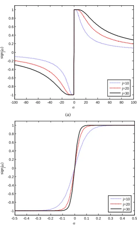
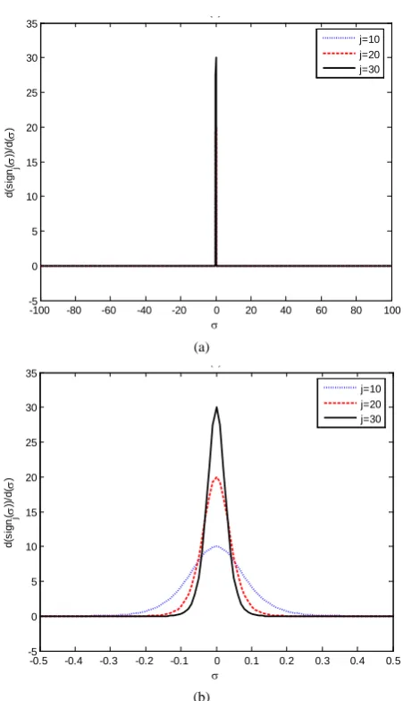
Figure 1(a) gives a big scope of the evaluated ap- proximated scalar sign function (9) for different values of j, and Figure 1(b) shows the figure detail near zero. The corresponding derivative (13) is shown in Figure 2(a) and the figure detail near zero in Figure 2(b). It can be found from Figure 1 that the larger the value of j is, the closer the curve of the approximated scalar sign function (9) approaches the one of the scalar sign function (11), so j is also called the approximation order in the following context. Figure 2 shows that the approximated scalar sign function (9) is differentiable everywhere because its derivative value is always finite with the largest one lo- cated at σ = 0, equal to the approximation order j.

By utilizing the approximated scalar sign function, an approximate model can be obtained for a non-smooth

(a)

[image:3.595.312.536.78.451.2]

(b)

Figure 1. Approximated scalar sign function.

dynamical system with sign function constraints, whose approximation accuracy can be adjusted with the ap- proximation order j. Due to the smoothness and nonli- nearity of the approximated scalar sign function, the re- sulting approximate model is still nonlinear, but differen- tiable everywhere, which makes possible the further local linearization.

Remark 1: As shown in Figure 1, sign_j

( )

σ ≤1 for j is even. This property will be exploited in the proposed anti-windup method in Section IV.

B) Optimal Linearization

Local linearization is a typical way of handling nonli- near systems and the most popular technique is Jacobian linearization [19]. However, as pointed out in [17,20], Jacobian Linearization usually produces an affine rather than linear model even at the equilibrium operating point. The only exception case is that the operating point is an equilibrium at the origin, which cannot be ensured through- out a nonlinear control process.

In order to circumvent the limitation of Jacobian linea- rization, Teixeira and Zak formulated linearization prob-

-100 -80 -60 -40 -20 0 20 40 60 80 100 -1

-0.8 -0.6 -0.4 -0.2 0 0.2 0.4 0.6 0.8 1

σ

s

ign

j

(σ

)

j=10 j=20 j=30

-0.5 -0.4 -0.3 -0.2 -0.1 0 0.1 0.2 0.3 0.4 0.5 -1

-0.8 -0.6 -0.4 -0.2 0 0.2 0.4 0.6 0.8 1

σ

s

ign

j

(σ

)

(a)

[image:4.595.59.285.76.468.2]

(b)

Figure 2. Derivative of approximated scalar sign function.

lem as a convex constrained optimization problem and proposed an optimal linearization approach in [17]. Ac- cording to this approach, an optimal local linear model can be achieved at any operating point, which possesses the exact dynamics of the original nonlinear system at the operating point and minimum approximation error (in the least square sense) in the neighborhood of that point. Due to the space limit, only the final conclusions are briefed below.

Consider a general class of nonlinear system in the form

( )

(

( )

)

(

( )

)

( )

x t = f x t +G x t u t (14) where x t

( )

∈ℜn is the state vector, u t

( )

∈ℜm is the input vector, f

( )

⋅ ℜ → ℜ: n with f

( )

0 =0 is a diffe- rentiable nonlinear function vector and G

( )

⋅ ℜ → ℜ: m n

is a function matrix. Its optimal local linear model at an arbitrary operating point x_k is in the state-space form

( )

k

( )

k

( )

x t =A x t +B u t (15)

where

( )

( )

( )

( )

T 2

2

for 0

0 for 0

k k k

k k k

k k

k

f x f x x

f x x x

x A

f x

 − ∇

∇ + ≠

 = 

∇ =



(16)

( )

k k

B =G x (17)

( )

k f x

∇ is the Jacobian matrix of f x

( )

evaluated at the operating point xk. It is noted that the case for xk= 0 in (16) agrees with the aforementioned exception case of the operating point being an equilibrium at the origin.

Remark 2: When f(x) in (14) is a scalar nonlinear func- tion, (16) is reduced to a scalar number as

( )

( )

for 0

0 for 0

k k k

k

k

f x x x

A

f x

 ≠



=  _′

=

 .

C) Analog Linear Quadratic Regulator

Together with a linear output equation, the linearized state Equation (15) constitutes a complete local linear model as

( )

k

( )

k

( )

x t =A x t +B u t (18a)

( )

( )

y t =Cx t (18b) where y t

( )

∈ℜp is the controlled output vector and

p n

C∈ℜ × is a constant matrix. According to LQR [21], if the linear system (18) is both controllable and observ- able, the optimal control law to minimize the perfor- mance index

( ) ( )

( ) ( )

( ) ( )

{

T _T

}

0 d

J=

∫

∞ _Cx t −r t _ Q Cx t_ −r t _+u t Ru t t

(19)

with Q≥0 and R>0, is then given by

( )

ck

( )

ck

( )

u t = −K x t +E r t (20) where

1 T

ck k k

K =R B P− (21)

(

)

₁ T

1 T T

ck k k k ck

E = −R B− _ A −B K − _ C Q (22)

r(t) is the reference for the controlled output y(t) to track, and Pkis the positive definite and symmetric solu- tion of the Ricatti equation

T 1 T T

0 k k k k k k k k

A P +P A −P B R B P− +C QC= (23) The weighting matrices Q and R should be tuned to make the resulting analog controller (20) give a desired control performance in the delay-free case.

3. Digital Redesign with Delay

Compensation

For time-delayed systems where delays can be caused by -100 -80 -60 -40 -20 0 20 40 60 80 100

-5 0 5 10 15 20 25 30 35

σ

d(

s

ign

j

(σ

))/

d

(σ

)

( )

j=10 j=20 j=30

-0.5 -0.4 -0.3 -0.2 -0.1 0 0.1 0.2 0.3 0.4 0.5 -5

0 5 10 15 20 25 30 35

σ

d(

s

ign

j

(σ

))/

d

(σ

)

( )

network transmission, controller computation, A/D and D/A conversions etc, a delay compensating technique is proposed next based on global digital redesign. Com- pared with the conventional digital redesign methods that the conversion is limited in the scope of the controller, like the bilinear transformation s=2

(

z−1

)

_T z

(

+1

)

_ [22], closed-loop global digital redesign techniques take into account the closed-loop nature of the whole control system, so the resulting digital controller is able to main- tain the essential performance of the analog counterpart even with a low sampling frequency [20,23-25].

For a Single-Input-Single-Output (SISO) plant, the time delays in a control loop from network transmission, controller computation, A/D and D/A conversions, sens- ing and actuation etc, can be combined and then allo- cated to either the input or the output side of the plant for control design purpose [26]. The input side is used in this paper, so the local linear model (15) is modified to in- clude the time delays as

( )

k

( )

k

(

)

x t =A x t +B u t−τ (24) where τ is the combined input delay. Among global digi- tal redesign methods, the prediction-based digital rede- sign in [20] reduces the conversion errors by shifting the digital control signal to defined inter-sampling instant, which is readily extendable for input delay compensation. This method is briefly introduced as follows and then extended to develop the proposed digital controller fea- turing the input delay compensation.

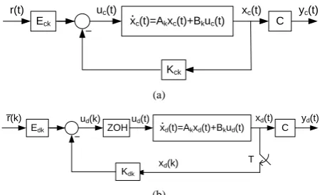
The analog linear plant (18) and the analog control law (20) constitute a complete analog control system as de- picted in Figure 3(a) where the subscript c is intended to differ from the following equivalent hybrid system which is subscripted with d. Suppose the equivalent hybrid sys- tem as depicted in Figure 3(b) and formulated by

( )

( )

( )

d k d k d

x t =A x t +B u t (25a)

( )

( )

d d

y t =Cx t (25b)

( )

( )

( )

d dk d dk

u kT = −K x kT +E r kT (25c) where the analog control input u_d

( )

t is a piecewise- constant signal generated from the digital control input

( )

d

u kT through Zero Order Hold (ZOH) as

( )

( )

d d

u t =u kT for kT≤ ≤t

(

k+1

)

T , and the digital state xd(kT) is the sample of the analog state xd(t) at the sampling instant t = kT; T is the sampling/control period. Equation (25c) is the digital control law to be designed so that the closed-loop state x_d

( )

t in the hybrid system can closely match the closed-loop state x t_c

( )

in the analog system at defined inter-sampling instant.

The solution x t_c

( )

of (18a) at t= =t_v kT+vT for 0≤ ≤v 1 is

(a)

[image:5.595.311.538.84.221.2]

(b)

Figure 3. Analog control system and its equivelent hybrid

cotnrol system.

( )

(

) ( )

(

)

( )

( )

_{( )}

( )

_{( )}

exp

exp d

c v k c

kT vT

k k c v

kT

v v

k c k c v

x t A vT x kT

A kT vT B u t

G x kT H u t

λ λ

+ ≈

+ _ + − _

= +

∫

(26)

where u t_c

( )

_v is a piecewise-constant input,

( )v _exp

₍

₎

k k

G = A vT

and

( )

₍

₎

( )

(

)

1

exp d

kT vT v

k _kT k k

v

k n k k

H A kT vT B

G I A B

λ λ

+

−

= _ + − _

= −

∫

,

in which I_n is an identity matrix of appropriate dimen- sion. The solution x_d

( )

t of (25a) at t=t_v is

( )

(

) ( )

(

)

( )

( )

_{( )}

( )

_{( )}

exp

exp d

d v k d

kT vT

k k d

kT

v v

k d k d

x t A vT x kT

A kT vT B u kT

G x kT H u kT

λ λ

+ =

+ _ + − _

= +

∫

(27)

Comparing (27) with (26) yields that with the assump-tion of x_d

( )

kT =x kT_c

( )

, the condition of

( )

( )

d v c v

x t =x t is u_d

( )

kT =u t_c

( )

_v , which leads to the prediction-based digital controller

( )

( )

( )

( )

( )

( )

d c v ck c v ck v

ck d v ck v

u kT u t K x t E r t

K x t E r t

= = − +

= − + (28)

By substituting (27) into (28), u_d

( )

kT is solved as

( )

(

( )

)

1 ( )

_{( )}

_{( )}

v v

d m ck k ck k d ck v

u kT = I +K H − _−K G x kT +E r t _ (29)

where I_m is an identity matrix of appropriate dimension. As a result, the desired digital control law (25c) is found from (29) having digital control gains

( )

(

)

1 ( )

v v

dk m ck k ck k

K I K H K G

−

= + (30a)

( )

(

)

1

v

dk m ck k ck

E I K H E

−

= + (30b)

r(t) Eck

uc(t)

xc(t)=Akxc(t)+Bkuc(t)

xc(t) yc(t)

Kck

C

.

r(k) Edk

ud(k)

ZOH xd(t)=Akxd(t)+Bkud(t)

xd(t) yd(t)

Kdk

xd(k) T

C

.

and the digital reference r kT

( ) (

=r kT+vT

)

. The pa- rameter v can be tuned to adjust the control performance.

Next, the conclusion in (28) will be extended for the input delay compensation. Considering the combined input delay τ, the state equation (25a) in the hybrid sys-tem is changed to

( )

( )

(

)

d k d k d

x t =A x t +B u t−τ (31) In order to compensate the input delay, the digital con-trol input u_d

( )

kT in (28) should be further predicted for the delay duration τ as

( )

(

)

(

)

(

)

d c v ck d v ck v

u kT =u t +τ = −K x t +τ +E r t +τ (32) where the future state x_d

(

t_v+τ

)

needs to be predicted based on the available signals x_d

( )

kT and u_d

( )

kT .

Compared with the sampling/control period, the time delays from controller computation, A/D and D/A con- versions etc, are relatively small, so a reasonable as- sumption is made in the following reasoning for simplic- ity purpose that the total duration of time delays in the control loop should not be larger than a sampling period, i.e. the combined input delay τ≤T . As for the case that

T

τ> , the proposed method can still handle but will produce a more complicated controller structure.

Let T

τ

σ = , so 0≤ ≤σ 1 and τ σ= T . The solution

( )

d

x t of (31) at t= +t_v τ is

(

)

(

)

( )

_{( )}

( )

₍

₎

( )

_{( )}

1

0

1

d v d

v v

k d k d

v

k d

x t x kT v T

G x kT H u k T

H u kT

σ σ

σ

τ σ

+ +

+

+ = _ + + _

= + _ − _

+

(33)

where

(v ) _exp

₍

₎

k k

G +σ = _A v+σ T_ , H₀(v_k+σ)=

(

G_k( )v −I_n

)

A B_k−1 _k

and ( )

(

( ) ( )

)

1

1

v v v

k k k k k

H +σ = G +σ −G A B− .

By substituting (33) into (32), u_d

( )

kT is solved as

( )

(

( )

)

{

( )

_{( )}

( )

₍

₎

₍

₎

}

1

0

1 1

v v

d m ck k ck k d

v

ck k d ck v

u kT I K H K G x kT

K H u k T E r t

σ σ

σ _τ

−

+ +

+

= + −

− _ − _+ + (34)

As a result, the desired digital controller for input de- lay compensation is derived from (34) as

( )

( )

(

1

)

( )

d dk d dk d dk

u kT = −K x kT −D u _ k− T_+E r kT (35)

where

( )

(

)

1 ( )

0

v v

dk m ck k ck k

K = I +K H +σ − K G +σ (36a)

( )

(

)

1 ( )

0 1

v v

dk m ck k ck k

D = I +K H +σ − K H +σ (36b)

( )

(

)

1

0 v

dk m ck k ck

E I K H σ E

− +

= + (36c)

and r kT

( ) (

=r t_v+τ

)

=r kT_ +

(

v+σ

)

T_. The result- ing hybrid control system has the configuration as shown in Figure 4. It is noted that for τ = 0, i.e. in the delay-free case, (35) agrees with the prediction-based digital control law (25c) as Ddk=0. Therefore, the prediction-based

digital redesign can be taken as a special case of pro- posed delay-compensating digital redesign.

4. Iterative Procedure for Anti-windup

Control

Consider a general nonlinear plant

( )

(

( )

)

(

( )

)

( )

c c c c

x t = f x t +G x t u t (37a)

( )

( )

c c

y t =Cx t (37b) where the symbols are defined as in (14) and (18b),

( )

m c

u t ∈ℜ is the true input vector whose i-th entry has the constraints

( )

( )

( )

( )

( )

max , max

, min , max

min , min

if

if

if

i i i

c ideal

i i i i i

c c ideal c ideal

i i i

c ideal

U u t U

u t u t U u t U

U u t U

 >



= ≤ ≤

 _<



(38)

for i=1, 2,,m, in which u_{c ideal}i_,

( )

t ∈ℜ is the ideal i-th input and U_maxi ,U_mini ∈ℜ are the top and bottom limits for the i-th input, respectively. For the purpose of simplicity, let _Umaxi _{= −Umin}i _>0 _{in the following} rea-soning. Through the optimal linearization in Section 2, the optimal local linear model of the nonlinear plant (37) at the k-th sampling instant is obtained as

( )

( )

( )

c k c k c

x t =A x t +B u t (39a)

( )

( )

c c

y t =Cx t (39b) where

(

A B_k, _k

)

are given by (16) and (17), respectively. Should no input saturation occur, i.e. i_,

( )

_maxi

c ideal

u t ≤U

for i=1, 2,,m , the state equation (39a) becomes

( )

( )

,

( )

c k c k c ideal

x t =A x t +B u t as u t_c

( )

=u_{c ideal,}

( )

t . Whenever input saturation happens, say, the i-th ideal input ui_{c ideal,}

( )

t is out of limits, the state Equation (39a) becomes

Figure 4. Proposed control scheme for input delay compen-

sation. r(k)

Edk

ud(k)

ZOH xd(t)=Akxd(t)+Bkud(t)

xd(t) yd(t)

Kdk

xd(k) T

C

.

e-sτ z-1

Ddk

( )

( )

( )

( )

( )

(

)

( )

1 , 2 , max , , c ideal c ideal

c k c k i i

c ideal

m c ideal

u t

u t

x t A x t B

U sign u t

u t           = +              (40)

which is apparently non-smooth due to the scalar sign function. Substituting approximated scalar sign function (9) for sign u

(

_{c ideal}i_,

( )

t

)

yields an approximated equation as

( )

( )

max

(

,

( )

)

...

...

i i

c k c k j c ideal

x t A x t B U sign u t

 

 

≈ + _{ }

 

 

 (41)

Equation (41) is still nonlinear due to

( )

(

,

)

i j c ideal

sign u t which can be further linearized by Remark 2 as

( )

(

)

(

,

_{( )}

( )

)

( )

, ,

, i j c ideal

i i

j c ideal i c ideal

c ideal sign u kT

sign u t u t

u kT     ≈    

where ,

( )

i c ideal

u kT is the k-th operating point of

( )

, i c ideal

u t . In this way, the non-smooth saturation Equa- tion (41) is fully linearized as

( )

( )

( )

( )

( )

( )

( )

( )

( )

( )

1 , 2 , , , , , , c ideal c ideal

c k c k i

k i c ideal

m c ideal

k c k k c ideal k c k c ideal

u t

u t

x t A x t B

u t

u t

A x t B u t A x t B u t

κ κ           ≈ +           = + = +    (42) where

( )

(

)

( )

, , max , i j c ideal i

k i i

c ideal sign u kT U

u kT

κ =  

 

 

,

,

diag 1,1, , , ,1

k k i

m

κ = _ κ _

 

  

and B_k =B_kκ_k. κ_k is called input scaling factor. To prevent the i-th input from saturation at t = kT, the input scaling factor κ_k should be tuned such that

( )

( )

, , , , max

i i i

k i c ideal k i c ideal t kT

u t u kT U

κ κ

= = ≤ , that is

( )

(

)

( )

( )

( )

(

)

, max , ,

max , max

i j c ideal

i i

c ideal i

c ideal

i i i

j c ideal

sign u kT

U u kT

u kT U sign u kT U

        = ≤ .

As mentioned in Remark 1, sign_j

( )

σ ≤1 for j is even, so the approximation order j is always an even number in the proposed anti-windup design.

From the linear state Equation (42), the input matrix

k

B is required for designing the ideal control input

( )

, c ideal

u t , while the input scaling factor κ_k, which de-termines B_k, involves the ideal control input u_{c ideal,}

( )

t at t=kT which has not been designed yet. To break this deadlock, a pre-designed control input is used to estimate

k

B which is then utilized to design the true control input. For a sampled-data control system, a pre-designed digital control input can be used for this purpose. As a result, the linear state Equation (42) is modified to

( )

( )

( )

( )

( )

, , ˆ ˆ

c k c k k c ideal

k c k c ideal

x t A x t B u t

A x t B u t

κ

≈ +

= +



(43)

where the estimated input matrix ˆB_k =B_kκˆ_k , the esti- mated input scaling factor ˆ_k diag 1,1, ,ˆ_{k i,}, ,1

m

κ =  κ 

       with

( )

(

)

( )

( )

( )

(

)

(

( )

)

( )

(

)

(

( )

)

, , max , , , max , _{, ,} ˆ 1 1 1 1 i j d ideal i

k i i

d ideal

j j

i i

i

d ideal d ideal

i j j

i i

d ideal _{d ideal d ideal}

sign u kT

U

u kT

u kT u kT

U

u kT _{u kT u kT}

κ = + − −   = _   + + −   (44)

for j is even. u_{d ideal}i_,

( )

kT is the pre-designed digital control input which can be the digitally redesigned con- trol input for the i-th component of u_{c ideal,}

( )

t at t = kT from the prediction-based digital redesign (25c) or the proposed delay-compensating digital redesign (35). With arbitrary input elements saturated, the state Equation (43) is generalized as

( )

( )

( )

( )

( )

, , ˆ ˆ

c k c k k c ideal

k c k c ideal

x t A x t B u t

A x t B u t

κ

≈ +

= +



(45)

with κˆ_k =diag

{ }

κˆ_{k i,} for i=1, 2,,m, where κˆ_{k i,} =1 or is given by (44) depending on whether the corres-ponding ideal input violates the constraints or not.

The general saturated state Equation (45) and the out- put Equation (39b) form a saturated system with mod-ified system matrices

(

A B Ck,ˆk,

)

. Applying LQR (21-23)

to it yields that with weighting matrices (Q, R), the op-timal control law is determined by solving the Riccati equation

T_{ˆ ˆ ˆ ˆ} 1_{ˆ ˆ}T T ₀

k k k k k k k k

A P +P A −P B R B P− +C QC= (46) which can be rewritten as

T_{ˆ ˆ ˆ ˆ} 1 T_ˆ T

0 k k k k k k k k

( )

( )

( )

, ˆ ˆ

c ideal ck c ck

u t = −K x t +E r t (48)

where the feedback gain

1 T 1 1 T 1

ˆ ˆ ˆ _ˆ ˆ ˆ _ˆ

ck k k k k k k ck

K =R B P− =κ−R B P− =κ−K

with _ˆ 1 T_ˆ

ck k k

K =R B P− , and the forward gain

(

)

(

)

T 1

1 T T

T 1

1 1 T T 1

ˆ ˆ ˆ ˆ

ˆ

ˆ ˆ

ck k k k ck

k k k k ck k ck

E R B A B K C Q

R B A B K C Q E

κ κ

− −

−

− − −

 

= − _ − _

 

 

= − _ − _ =

 

with

(

)

T 1

1 T T

ˆ

ck k k k ck

E = −R B− _ A −B K − _ C Q

  .

On the other hand, applying LQR to the original sys- tem

(

A B C_k, _k,

)

in (39) with the modified weighting pair

( )

_{Q R,}ˆ _{yields the optimal control law}

( )

( )

( )

c ck c ck

u t = −K x t +E r t (49) where the feedback gain K_ck and the forward gain E_ck are shown above. The corresponding Riccati equation is the same as (47).

It can be observed by comparing the above two LQR designs that the problem of finding the optimal control law for the saturated system (45) with the weighting ma- trices (Q, R) can be reformulated as the same problem for the original system (39) using the same performance in- dex (19), but with the new weighting matrices

( )

Q R,ˆ

where _{ˆ ˆ} 1 _ˆ 1

k k

R=κ−Rκ− . Generally, both weighting matrices are selected to be positive definite diagonal matrices. So when the input scaling factor’s i-th diagonal element

, ˆ_{k i} 1

κ < , the corresponding i-th diagonal elements of R and Rˆ have the relationship of Rˆi κˆk i,1Riκˆk i,1 Ri

− −

= > . As

the matrix Q is kept the same in the performance index, the resulting control law u_{c ideal,}

( )

t with

( )

Q R,ˆ will have a smaller i-th element than the counterpart with (Q, R). Accordingly, the corresponding i-th element of digi-tally redesigned control input u_{d ideal,}

( )

t would be smaller as well, thus possibly avoiding input saturation. It is noted that although ˆR_i is 2

,

ˆ_{k i}

κ− _{times greater than}

Ri, the newly resulting digital input ,

( )

i d ideal

u t is not

necessarily κˆ_{k i}−_,2 times smaller than the original one and may be still out of input limits after a single update. Therefore, it might be necessary to recursively update on

ˆ i

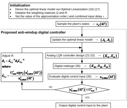
R until the input lies within the saturation limits. Fig- ure 5 summarizes the general steps of proposed anti- windup digital controller design for analog nonlinear system with input constraints. The digital redesign adopted is the proposed delay-compensating technique, so besides the anti-windup functionality, the proposed digital controller can also survive in a time-delayed en- vironment.

[image:8.595.313.537.82.271.2]

Remark 3: The approximation order j in the approx- imated scalar sign function can be tuned to achieve cer- tain tradeoff between the control performance and the recursion efficiency. As shown in Figure 1, a smaller

Figure 5. Anti-windup plus delay-compensating digital con-

troller.

approximation order j leads to a faster decaying approx- imated scalar sign function, which results in a smaller

, ˆ_{k i}

κ . This can be regarded as an ‘aggressive’ update scheme with the advantage that a smaller number of ite- rations are needed for suppressing the input to within the limits. But the disadvantage is that the input could be suppressed too much below the limit, which may bring a fairly slow system response.

5. Simulation Results

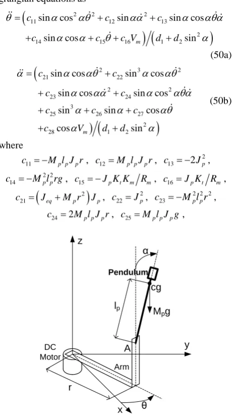
As a typical nonlinear system, the rotary inverted pendu- lum system depicted in Figure 6 presents many chal- lenging topics for investigation, like coupling, underac- tuation, instability, multivariable, time-sensitivity etc. The pendulum control can be simply categorized into swing-up (the motor drives the L-shaped arm to swing the pendulum up to around the upright position) and sta- bilization (the motor drives the arm to stabilize the pen- dulum at the upright position). Nonlinear control me- thods are usually proposed for swing-up control while LQR is commonly used for stabilization control. The failure to apply LQR on swing-up control results from the deficiency of traditional linearization method which only works around the equilibrium points while the pen-dulum is running in off-equilibrium region in swing-up process. In the proposed anti-windup design, the optimal linearization approach is utilized to obtain the local linear model at any operating point, and then LQR is applied to produce a state-feedback controller optimal for each op- erating point. Therefore, the proposed design can be ap- plied throughout both swing-up and stabilization pro- cesses, avoiding the trouble of switching controllers in conventional methods.

The dynamics between the arm angle θ, the pendulum angle α and the motor voltage Vm is derived using La-

Initialization

• Derive the optimal linear model via Optimal Linearization (16) (17). • Initialize the weighting matrices Q and R.

• Set the value of the approximation order j and combined input delayτ.

Output digital control input to the plant Sample the plant’s states →

Analog LQR controller design (21-23) →

Evaluate digital control input (35) →

YES NO

Proposed anti-windup digital controller

Digital redeisgn (36) → Update the optimal linear model →

grangian equations as

(

) (

)

2 2 2

11 12 13

2

14 15 16 1 2

sin cos sin sin cos

sin cos _m sin

c c c

c c c V d d

θ α αθ αα α αθα

α α θ α

= + +

+ + + +

  _ _



(50a)

(

)

(

)

2 3 2

21 22

2 2

23 24

3

25 26 27

2

28 1 2

sin cos sin cos

sin cos sin cos

sin sin cos

cos m sin

c c

c c

c c c

c V d d

α α αθ α αθ

α αα α αθα

α α αθ

α α

= +

+ +

+ + +

+ +

 





 

 (50b)

where

11 p p p

c = −M l J r, c₁₂ =M l J r_{p p p} , c13= −2Jp2, 2 2

14 p p

c = −M l rg, c₁₅= −J K K_{p t m} R_m, c₁₆=J K_{p t} R_m,

(

2

)

21 eq p p

c = J +M r J , 2 22 p

c =J , 2 2 2

23 p p

c = −M l r ,

24 2 p p p

[image:9.595.58.288.93.504.2]

c = M l J r, c₂₅=M l J g_{p p p} ,

Figure 6. Single rotary inverted pendulum.

(

2

)

26 eq p p p

c = J +M r M l g, c₂₇ =M l rK K_{p p t m} R_m,

28 p p t m

c = −M l rK R , d₁=J J_{eq p}+M r J_p 2 _p −M l r_{p p}2 2 2, 2 2 2 2

2 p p p

d =J +M l r .

[image:9.595.50.539.547.735.2]

The parameters have physical meanings defined in Table 1 as well as their values used in the following si- mulations. Apparently, (50) is highly nonlinear and cou- pled expressions.

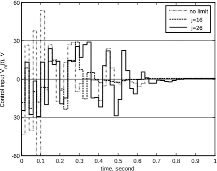
For space-saving purpose, the derivation of optimal local linear model of (50) is skipped, and only salient simulation results and necessary explanations are pre- sented here. The proposed anti-windup methodology in Figure 5 was implemented in simulations with the initial pendulum angle of 179˚ (almost the downward position), the initial weighting matrices Q = diag{50, 0, 1, 0} and R = 1, and the digital control period T = 0.01 s. Figure 7 compares the simulated control performances of pro- posed method under no input limit and the limits ±30 V with different approximation order j. The corresponding control inputs are shown in Figure 8. Obviously, the freely redesigned digital control voltage in Figure 8 is out of the limits ±30 V over multiple control periods; using the proposed anti-windup method, whatever the value of j is, the control voltage is successfully sup- pressed to within the specified limits ±30 V. Another apparent fact is that over the first few control periods, the control voltage for j = 16 is suppressed more than the one for j = 26, which results in a little slower control perfor- mance in Figure 7. This echoes the claims by Remark 3. No time delay is introduced in the control loop in this case, so the proposed delay-compensating digital control law (35) converges to the prediction-based digital control law (25c) and the parameter v is set to 1.

Next, an input time delay is introduced between the pendulum’s motor and the digital controller to represent

Table 1. Single rotary inverted pendulum nomenclature.

Symbol Description Value Unit

Mp Mass of the pendulum assembly (weight and link combined). 0.027 kg

lp Length of pendulum center of gravity from pivot. 0.156 m

r Length of arm pivot to pendulum pivot. 0.0826 m

Jeq Equivalent moment of inertia about motor shaft pivot axis. 1.23e−4 kg∙m2

Jp Pendulum moment of inertia about its pivot axis. 7.3e−4 kg∙m2

Rm Motor armature resistance. 3.3 Ω

Kt Motor torque constant. 0.02797 N∙m

Km Motor back-electromotive force constant. 0.02797 V/(rad/s)

g Gravitational acceleration constant. 9.81 m/s2

z

x

y

r

lp

A cg

Mpg

θ α

Pendulum

Arm DC

[image:10.595.67.281.84.253.2] [image:10.595.310.535.86.260.2]

Figure 7. Control performance of proposed design in the delay-free case.

Figure 8. Control inputs of proposed design in the delay-

free case.

the potential time delays in the real-world control loop. In order to demonstrate the delay-compensating capabil- ity, a reasonably long time delay τ = 0.02 s is used. The control period T is accordingly extended to 0.02 s as the proposed design assumes a control period no shorter than the delay duration. Other parameters and initial condi-tions are the same as the delay-free case. Simulation re-sults showed that the controller from the prediction-based digital redesign cannot succeed any more, exhibiting an unstable behavior. In contrast, the proposed anti-windup plus delay-compensating controller can still survive with performances shown in Figure 9. Figure 10 depicts the evolutions of control inputs: the motor voltages in con-strained cases are successfully suppressed to within the desired range. Hence, the efficacy of proposed design is well demonstrated.

6. Conclusions

[image:10.595.66.278.293.457.2]

This paper describes the design and application of an

Figure 9. Control performance of proposed design in the

delayed case.

Figure 10. Control inputs of proposed design in the delayed

case.

optimal anti-windup digital controller for analog nonli- near plants subject to input constraints. As a new anti- windup technique for sampled-data control systems, the proposed method has the following contributions: 1) the approximated scalar sign function is utilized to model non-smooth input saturations, which presents a new ef- fective solution to sign-function constrained non-smooth problems; 2) through the optimal linearization, a general approach is developed for handling nonlinear systems with linear control theories in a broader region instead of conventionally being limited to around equilibriums; 3) aside from the anti-windup functionality, the proposed digital controller is capable of compensating time delays in the control loop, which would help guarantee its de- signed performance in real world implementations.

Funding

Research supported by NSF award #1238859, and De-

0 0.5 1 1.5

-20 0 20 40 60 80 100 120 140 160 180

time, second

P

endul

um

angl

e α

(t

),

degr

ee

no limit j=16 j=26

0 0.1 0.2 0.3 0.4 0.5 0.6 0.7 0.8 0.9 1 -90

-60 -30 0 30 60 90

time, second

M

ot

or

v

ol

tage V

m

(t

),

V

no limit j=16 j=26

0 0.5 1 1.5

-20 0 20 40 60 80 100 120 140 160 180

time, second

P

endul

um

angl

e α

(t

),

degr

ee

no limit j=16 j=26

0 0.1 0.2 0.3 0.4 0.5 0.6 0.7 0.8 0.9 1 -60

-30 0 30 60

time, second

C

ont

rol

i

nput

V

m

(t

),

V

[image:10.595.312.535.302.477.2]

partment of Education, HBGI Grant.

REFERENCES

[1] M. V. Kothare, P. J. Campo, M. Morari and C. N. Nett, “A Unified Framework for the Study of Antiwindup De- signs,” Automatica, Vol. 30, No. 12, 1994, pp. 1869-1883. http://dx.doi.org/10.1016/0005-1098(94)90048-5

[2] C. Edwards and I. Postlethwaite, “Anti-Windup, Bump- less-Transfer Schemes,” Automatica, Vol. 34, No. 2, 1998, pp. 199-210.

http://dx.doi.org/10.1016/S0005-1098(97)00165-9 [3] P. Westen and I. Postlethwaite, “Linear Conditioning for

Systems Containing Saturating Actuators,” Automatica, Vol. 36, No. 9, 2000, pp. 1347-1354.

http://dx.doi.org/10.1016/S0005-1098(00)00044-3 [4] Y. S. Chen, J. S. H. Tsai, L. S. Shieh and F. C. Kung,

“New Conditioning Dual-Rate Digital-Redesign Scheme for Continuous-Time Systems with Saturating Actuators,”

IEEE Transactions on Circuits and Systems I: Funda- mental Theory and Applications, Vol. 49, No. 12, 2002, pp. 1860-1870.

http://dx.doi.org/10.1109/TCSI.2002.805731

[5] V. R. Marcopoli and S. M. Phillips, “Analysis and Synthe- sis Tools for a Class of Actuator-Limited Multivariable Control Systems: A Linear Matrix Inequality Approach,”

International Journal of Robust and Nonlinear Control, Vol. 6, No. 9-10, 1996, pp. 1045-1063.

http://dx.doi.org/10.1002/(SICI)1099-1239(199611)6:9/1 0<1045::AID-RNC268>3.0.CO;2-S

[6] E. F. Mulder, M. V. Kothare and M. Morari, “Multivaria- ble Anti-Windup Controller Synthesis Using Linear Ma- trix Inequalities,” Automatica, Vol. 37, No. 9, 2001, pp. 1407-1416.

http://dx.doi.org/10.1016/S0005-1098(01)00075-9 [7] G. Grimm, J. Hatfield, I. Postlethwaite, A. R. Teel, M. C.

Turner and I. Zaccarian, “Anti-Windup for Stable Linear Systems with Input Saturations: A LMI Based Synthesis,”

IEEE Transactions on Automatic Control, Vol. 48, No. 9, 2003, pp. 1509-1525.

http://dx.doi.org/10.1109/TAC.2003.816965

[8] J. R. Calvet and Y. Arkun, “Feedforward and Feedback Linearization of Nonlinear Systems and Its Implementa- tion Using IMC,” Industrial & Engineering Chemistry Research, Vol. 27, No. 10, 1988, pp. 1822-1831.

http://dx.doi.org/10.1021/ie00082a015

[9] L. Del Re, J. Chapuis and V. Nevistic, “Predictive Control with Embedded Feedback Linearization for Bilinear Plants with Input Constraints,” Proceedings of the 43rd

IEEE Conference on Decision and Control, San Antonio, 15-17 December 1993, pp. 2984-2989.

[10]T. A. Kendi and F. J. Doyle, “An Anti-Windup Scheme for Multivariable Nonlinear System,” Journal of Process Control, Vol. 7, No. 5, 1997, pp. 329-343.

http://dx.doi.org/10.1016/S0959-1524(97)00011-5 [11]Q. Hu and G. O. Rangaiah, “Anti-Windup Schemes for

Uncertain Nonlinear Systems,” IEE Proceedings of Con- trol Theory and Applications, Vol. 147, No. 3, 2000, pp. 321-329. http://dx.doi.org/10.1049/ip-cta:20000136

[12]R. Bouc, “Forced Vibration of Mechanical Systems with hysteresis,” Proceedings of 4th Conference Nonlinear Os- cillation, Prague, 5-9 September 1967, p. 315.

[13]Y. K. Wen, “Method for Random Vibration of Hysteretic Systems,” Journal of Engineering Mechanics Division, 1976, pp. 249-263.

[14]B. Jacobson, “The Stribeck Memorial Lecture,” Tribology International, Vol. 36, 2003, pp. 781-789.

[15]L. S. Shieh, Y. T. Tsay and R. Yates, “Some Properties of Matrix Sign Functions Derived from Continued Fractions,”

IEEE Proceedings of Control Theory and Applications, Part D, Vol. 130, 1983, pp. 111-118.

[16]L. S. Shieh, Y. T. Tsay and C. T. Wang, “Matrix Sector Functions and Their Applications to Systems Theory,”

IEEE Proceedings of Control Theory and Applications, Part D, Vol. 131, 1984, pp. 171-181.

[17]M. C. M. Teixeira and S. H. Zak, “Stabilizing Controller Design for Uncertain Nonlinear Systems Using Fuzzy Models,” IEEE Transaction on Fuzzy Systems, Vol. 7, No. 2, 1999, pp. 133-142.

http://dx.doi.org/10.1109/91.755395

[18]J. D. Roberts, “Linear Model Reduction and Solution of the Algebraic Riccati Equations by Use of the Sign Func- tion,” International Journal of Control, Vol. 32, No. 4, 1980, pp. 677-687.

http://dx.doi.org/10.1080/00207178008922881

[19]F. Esfandiari and H. K. Khalil, “Output Feedback Stabili- zation of Fully Linearizable Systems,” International Journal of Control, Vol. 56, No. 5, 1992, pp. 1007-1037. http://dx.doi.org/10.1080/00207179208934355

[20]S. M. Guo, L. S. Shieh, G. Chen and C. F. Lin, “Effective Chaotic Orbit Tracker: A Prediction-Based Digital Rede- sign Approach,” IEEE Transaction on Circuits and Sys- tems, Vol. 47, 2000, pp. 1557-1570.

[21]F. L. Lewis, “Optimal Control,” Wiley, New York, 1986.

[22]K. Ogata, “Discrete-Time Control Systems,” Prentice-Hall, Englewood Cliffs, 1987.

[23]J. S. H. Tsai, C. M. Chen and L. S. Shieh, “Digital Rede- sign of the Cascaded Continuous-Time Controller: Time- Domain Approach,” Control Theory Advanced Techni- ques,Vol. 17, 1991, pp. 643-661.

[24]L. S. Shieh, W. M. Wang and M. K. A. Panicker, “Design of PAM and PWM Digital Controllers for Cascaded Analog Systems,” ISA Transaction,Vol. 37, No. 3, 1998, pp. 201-213.

http://dx.doi.org/10.1016/S0019-0578(98)00026-3 [25]L. S. Shieh, J. L. Zhang and N. P. Coleman, “Optimal

Digital Redesign of Continuous-Time Controllers,”

Computers & Mathematics with Applications, Vol. 22, No. 1, 1991, pp. 25-35.

http://dx.doi.org/10.1016/0898-1221(91)90022-V [26] H. Wang, L. S. Shieh, Y. Zhang and J. S. Tsai, “Minimal

Realization of the Transfer Function Matrix with Multiple Time Delays,” IET Control Theory and Application, Vol. 1, No. 5, 2007, pp. 1294-1301.