Munich Personal RePEc Archive
Do all countries follow the same growth
process?
Davis, Lewis and Owen, Ann L. and Videras, Julio
Union College, Hamilton College
November 2007
Online at
https://mpra.ub.uni-muenchen.de/11589/
Do All Countries Follow the Same Growth Process?
Lewis Davis Union College [email protected]
Ann Owen* Hamilton College [email protected]
Julio Videras Hamilton College [email protected]
September 2008
Abstract
We estimate a finite mixture model in which countries are sorted into groups based on the similarity of the conditional distributions of their growth rates. We strongly reject the hypothesis that all countries follow a common growth process in favor of a model in which there are two classes of countries, each with its own distinct growth process. Group membership does not conform to the usual categories used to control for parameter heterogeneity such as region or income. However, we find strong evidence that one country characteristic that helps to sort countries into different regimes is the quality of institutions, specifically, the degree of law and order. Once institutional features of the economy are controlled for, we find no evidence that geographic characteristics play a role in determining the country groupings.
JEL Codes: O11, O17
Key words: finite mixture models, multiple equilibria, institutional quality
1 Introduction
Is there a universal growth model, a single set of equations that govern the evolution of per capita
income in every country or a majority of countries? And if not, is it possible to group countries in such a
way that, within each group, we are able to draw inferences about their common growth experience? Or
must we assume that each country’s growth experience is fundamentally idiosyncratic, a position
Hausmann, Rodrik and Velasco (2005:1) say results in an “attitude of nihilism” regarding our ability to
understand economic growth? As these questions suggest, addressing the heterogeneity of country
growth processes is of fundamental importance to the study of economic growth.
While most growth economists would agree that heterogeneity is an important consideration in
empirical work, the most common methods for addressing heterogeneous growth are unsatisfactory. For
example, the practice of including regional dummy variables or country fixed effects when panel data are
available controls for differences in average growth rates, but it does not allow for differences in the
marginal effect of the regressors. An alternative is to identify groups of countries for which the growth
process is assumed to be similar, for example, developed and developing country groups, but this
approach requires we choose an a priori income threshold and it may still result in groups with countries
that follow very different growth processes. This latter concern appears to underlie the further partition of
developing countries into regional subgroups such as African or Latin American countries.
In contrast to these somewhat ad hoc approaches, we employ a data-driven methodology to
estimate multiple growth processes. We estimate a finite mixture model in which countries are sorted
into groups based on the similarity of the conditional distributions of their growth rates. We model the
distribution of growth rates as a function of variables identified as proximate determinants of growth:
initial income, the rate of investment in physical capital, human capital, and the population growth rate.
We also extend our analysis to use variables that describe institutional and geographic factors to improve
the classification of countries into the different growth regimes.
Our results are as follows. First, we strongly reject the hypothesis that the countries in our
processes. Moreover, our parameter estimates differ significantly both across groups and from estimates
found in a standard growth regression that assumes only one class. Second, we show that classification
into the different growth regimes does not depend solely on categories such as income and region.
Therefore, finite mixture regression modeling can improve upon the standard treatment of dividing
countries by income level because it allows for parameter heterogeneity among countries with similar
incomes. Finally, we show that institutional factors play a clear role in predicting membership in the
country groups, but we find no evidence that geographic characteristics help to explain the country
groupings. For growth empirics, our results suggest a middle ground to the two extremes mentioned at
the start of the paper. All countries do not follow the same growth process, but neither is each country’s
growth process entirely unique. Our analysis shows that countries can be grouped in a meaningful way.
Our work is related to that of other researchers who have examined the heterogeneity of the
growth process with increasing methodological sophistication. In a seminal paper in this literature,
Durlauf and Johnson (1995) apply regression tree analysis to identify country groupings. These authors
use output per capita and adult literacy rates to identify countries with common growth processes.
Papageorgiou (2002) extends the work of Durlauf and Johnson (1995) by also exploring whether or not
trade can be used as a threshold variable. More recently, Canova (2004) and Sirimaneetham and Temple
(2006) have explored the existence of multiple growth regimes. Sirimaneetham and Temple (2006) use
principal components analysis to generate an index of policy quality, sort economies into groups based on
the value of the index, and then explore whether average growth rates vary across groups. Canova (2004)
draws on Bayesian ideas to examine income levels in Europe. His technique allows him to explore
alternative means of ordering countries to form groups and he finds that using initial income as a splitting
variable generates four groups of countries. Our research shares the same motivation of these papers but
our methodology complements and advances the existing literature. Contrary to Durlauf and Johnson
(1995), Papageorgiou (2002), Canova (2004), and Sirimaneetham and Temple (2006), we assign countries
to growth regimes based on the conditional distribution of the growth rate itself rather than predetermined
are discrete and unordered in the usual sense (i.e., the regimes are different, not necessarily better or faster
growing).
Bloom, Canning, and Sevilla (2003) use methods more similar to ours, finding evidence that a
model with two income regimes is statistically superior to a model with one regime. These authors also
argue that geographical variables determine the likelihood that a country is assigned to any of the two
regimes. However, unlike our work which focuses on the conditional distribution of growth rates, Bloom
et al. focus on the unconditional distribution of the level of income and do not consider the possibility of
more than two regimes. Like Bloom et al., we also explore the role of geography in determining the class
or regime to which a country belongs, but we find no evidence that geographic factors sort countries into
growth regimes once the quality of institutions is allowed to enter the estimation.
Paap, Franses, and van Dijk (2005) apply latent class models to a panel of countries allowing the
growth rates data to determine the number of groupings. They find that a model assuming three
groupings of countries is statistically superior to a model that assumes economies are homogeneous. In
this aspect, our methodology is similar to the work by Paap, Franses, and van Dijk (2005).1 However, this paper makes three additional original contributions. First, we examine growth rates in both
developed and developing economies, unlike Paap, et. al. who only examine growth in developing
countries. Second, by examining the conditional distribution of growth rates rather than the unconditional
distribution, we are able to estimate the marginal effects of growth fundamentals within regimes. For
example, we identify a group of countries for which initial income is negatively related to subsequent
growth and one in which it is positively related. Finally, and most importantly, our method allows us to
perform hypothesis testing on the sources of systematic heterogeneity that explain the assignment of
countries to specific latent regimes in a way that ties our empirical results into the current growth
literature.
1
Finally, the paper most closely related to our work is Alfo, Trovato and Waldmann (2008). As
we do, they estimate a finite mixture model on a panel of 5-year growth rates for a large set of countries.
They identify multiple growth regimes and speculate that the latent variable that defines the classes may
be related to institutions.2 Our analysis takes this as a starting point and extends the method employed by Alfo, et. al. by accounting for the sources of heterogeneity across countries. This methodology allows us
to test which factors affect the latent variable sorting countries into growth regimes. We show that the
quality of institutions does in fact help to predict the latent variable grouping countries. We are also able
to simultaneously test alternative hypotheses as suggested by Bloom, et. al. (2003) that geographic
characteristics determine growth regimes.
In comparing our work to the existing growth literature, we note that an important theme in both
the empirical and theoretical growth literature is the existence of multiple equilibria.3 Empirical estimation of models with multiple equilibria typically relies on using observable characteristics such as
income or education levels to sort countries into regimes. Our work is related to this approach, with an
important difference. Specifically, our methods allow us to sort countries into growth regimes based on
an unobservable latent variable that is determined by the conditional distribution of growth rates and
country characteristics that are often referred to as the “deeper determinants” of growth such as
institutions and geography. Therefore, we believe our work extends this line of thinking because we are
able to choose a number of country characteristics as indicators of the latent variable and statistically test
the validity of these indicators. Furthermore, while the existence of “convergence clubs” may be a result
of countries experiencing different growth processes, it does not necessarily have to be. Identifying these
clubs is not the goal of our analysis; we examine a much broader phenomenon. In fact, our results
suggest that conditional convergence occurs only within a subset of countries. For several countries in
2
Alfo, Trovato and Waldmann (2008) find more classes than we do. However, because we are interested in testing hypotheses about institutional quality, we restrict our sample only to those countries for which we have data on institutional quality. Therefore, our data set is somewhat smaller which results in fewer classes.
3
our sample, we do not find evidence that their incomes are converging to that of other countries in its
grouping.
The remainder of the paper is organized as follows. The following section provides a theoretical
framework for our results and discusses our choice of regressors and covariates. Section 3 presents our
econometric approach. Section 4 presents and discusses our empirical findings, and the final section
concludes.
2 Empirical Framework
The empirical model we estimate includes regressors that capture the proximate determinants of
economic growth. Investment, education, and population growth are direct measures of the growth of
productive factors. Initial income controls for transitional dynamics that occur when earlier gains are
easier than later ones, either due to technical transfer or diminishing marginal returns to capital. Our
estimations are based on a standard growth equation:
(1)
where gi,t is the 5-year average growth rate of real per capita income of country i in period t, is initial
income in period t, is the average investment rate, is the average years of education of the labor
force during the initial year of the period, ni,t is the average population growth rate over period t for
country i, g is the growth rate of technology and δ is the depreciation rate. Following Mankiw, Romer and
Weil (1992) we assume the annual rates of growth of technology and of depreciation are constant and
sum to .05. The constant term captures increases in labor productivity that are orthogonal to factor
accumulation and initial conditions.
As shown by Mankiw, Romer, and Weil (1992), this specification can be derived directly from a
Cobb-Douglas production function with capital, labor and human capital as inputs. We will estimate
Equation 1 with panel data. As will become clearer in Section 3, the technique that we describe below
help us to determine which countries can be grouped together. Admittedly, 5-year intervals may be the
minimum length of time that will allow us to comment on factors affecting longer-run growth and we
urge caution in interpreting the results. We discuss some attempts at applying this method to longer-term
growth rates in Section 4.
The model in Equation 1 deliberately lacks novelty. The regressors are those suggested by the
augmented neoclassical model employed by Mankiw, Romer and Weil (1992). They are also among the
handful of variables identified by Levine and Renelt (1992) as being robust determinants of economic
growth. While neither of these papers has gone unchallenged, they both exerted a large impact on later
growth empirics, allowing comparison of our results with other empirical work on growth.
As we explain in more detail below, we also employ covariates that are not direct determinants of
growth but help to sort countries into different growth regimes. This novel feature of our estimation
allows us to present empirical results that are more consistent with the idea that some variables are
proximate determinants of growth, while others may be considered “deeper” determinants in that they
influence the overall environment in which growth occurs. (e.g., Rodrik, Subramanian, and Trebbi, 2004)
In choosing our covariates, we focus on two categories of variables that the literature suggests play a
central role in determining a country’s growth process, and more particularly how it responds to capital
accumulation, population growth and the dynamics of convergence. We proceed by choosing broad
categories of country characteristics (institutions and geography) that have been suggested by a large
body of work and then choosing indicators within each category that capture important features of this
characteristic. An advantage of our approach is that it recognizes that these covariates are indicators of
class membership with error. In other words, our procedure recognizes that there is some error associated
with the process of assigning countries to classes and, as we discuss in the following section, we can
attempt to gauge the error associated with our country groupings.
As there is an immense literature related to each of our covariates, we mention only briefly some
of the previous work that motivated our choice to use measures of institutional quality and geography to
growth. (See, for example, Mauro (1995), Acemoglu, Johnson and Robinson (2001), Dollar and Kraay
(2003) and Rodrik, Subramanian and Trebbi (2004), among others.) Democratic political institutions in
particular may also affect the economics of accumulation with a central thesis in the theoretical literature
on democracy and growth being that populist policies may blunt incentives to invest in physical capital as
in Alesina and Rodrik (1994) and Persson and Tabellini (1994), while also potentially subsidizing the
accumulation of human capital as suggested by Bourguignon and Verdier (2000) and Benabou (2000).
Geography has also played a prominent role in the growth literature. As mentioned previously, in
an article closely related to ours, Bloom, Canning, and Sevilla (2003) find that countries with cool, coastal
locations have relatively high income, but that hot, landlocked countries with low rainfall are more likely
to be in a poverty trap. Their work follows a number of studies that have linked climate and geographic
features to economic performance. (See, Bloom and Sachs (1998), Sachs and Warner (1997) and Gallup,
Sachs and Mellinger (1999) as just a few examples of this previous literature.)
Because we chose these covariates based on their prominence in the growth literature, our
contribution to this literature is not to propose new growth determinants—it is to empirically model their
effect in a fundamentally different way. In other words, we do not model these covariates as direct
determinants of growth, but as indirect determinants that influence the environment in which growth
occurs and the marginal productivity of the growth fundamentals.
3 Method: Finite mixture regression model
We use a finite mixture approach to estimate the growth regression model in Equation 1. This
approach is an application of latent class regression models to estimate a latent discrete distribution of
growth regimes. Our approach has four important features. First, the observed conditional distribution of
growth rates is assumed to be a mixture of two or more distributions with different means and variances.
Second, the parameters of the growth regression are allowed to differ across regimes. Third, the
distribution of the latent regimes and the parameters of the growth regression for each regime are
estimated jointly. Finally, in addition to accounting for heterogeneity in the growth process, finite
whether indicators of institutional quality and geography can improve the model’s fit and the assignment
of countries to growth regimes.
Specifically, we assume that growth processes can be classified into M discrete classes. Letting T
represent the number of repeated observations per country, Z be the vector of independent variables in
Equation 1, and letting x indicate class membership, the probability structure for a given country is:
(2)
where is the probability of membership in latent class x and is the distribution of
growth rates conditional on membership in latent class x and independent variables. We assume the latent
variable follows a multinomial probability that yields a standard multinomial logit model:
(4)
where the linear predictor is such that membership in class m is defined by:
(5)
Under this formulation, we compare the probability of being assigned to class m with the
geometric average of the probabilities of all M classes.
We extend our analysis by examining the determinants of class membership. We use variables
related to the quality of institutions and geographic features as covariates that help predict class
membership. Denoting the vector of K covariates as V, we can now write the probability structure for a
model with covariates as:
(6)
This approach differs from the standard treatment in the literature because we treat these
countries into growth regimes based on the combination of these indicators rather than on the value of
specific indicators. Thus, our method is not simply a substitute for interacting the individual indicators
with the regressors.
Now, the probability of latent-regime memberships is:
(7)
and:
(8)
The model is estimated via maximum likelihood. In the case of the model with covariates,
maximum-likelihood estimation involves finding the estimates of the beta parameters and the vector of
gamma parameters that maximize the log-likelihood function derived from the conditional
probability density function in Equation 6. Assuming the error term in the growth rate equation comes
from a normal distribution and adding subscript i to identify countries, the log-likelihood function is:
=
(9)
where
and and are the mean and variance of the growth rate of the sub-population in class m. In the case
of the model without covariates, the log-likelihood function of the model is the same as in Equation 9 but
replacing with
We use Latent GOLD to perform the estimation. In practice, the likelihood functions for these
types of models can feature local maxima. To ensure that we obtain the global maximum, we estimate
each model using 10,000 sets of starting values. Each set might result in different log-posteriors. Latent
GOLD uses the best solution until convergence (Vermunt and Magidson, 2005). We repeat the process
twice to verify we obtain the same solution. In our application, we always obtain the same log likelihood
for the same estimations, making us confident that we are obtaining global maxima for the models.
We use the empirical Bayes rule to calculate country-specific posterior membership probabilities
for each country i = 1,…,N,
. (11)
Because all of the parameters in the likelihood function (described in Equations 7, 8, 9 and 10) are
estimated jointly, the posterior membership probabilities depend on both the value of the covariates and
the distribution of growth rates.
Equation 11 emphasizes a key advantage of the finite mixture approach: the probability of class
membership depends on the conditional distribution of growth rates and the covariates. Once we
calculate the probability of class membership for each country using Equation 11, we use the empirical
Bayes modal classification rule to assign countries into classes; that is, each country is assigned to the
class for which it has the largest posterior probability. Although for most countries the classification
occurs with posterior probabilities very close to 1, the classification is probabilistic. The quality of the
and the overall misclassification rate errors by
(Skrondal and Rabe-Hesketh, 2004).
In practice, the number of classes is unknown to the researcher. We start with a one-class model
and then estimate subsequent models that increase the number of classes by one each time. We use
information criteria based on the model’s log likelihood to select the model that best fits the data. We use
three different information criteria to evaluate the models: the Bayesian Information Critera (BIC), the
Corrected Akaike Information Criteria (CAIC) and the Akaike Information Critera 3 (AIC3). All three
criteria are decreasing in the value of the log likelihood and increasing in the number of parameters
estimated. Therefore, we choose the model with the lowest BIC, CAIC and AIC3. Specifically, the BIC=
-2LL + log(N)J, the CAIC=-2LL+log(N+1)J, AIC3=-2LL + 3J where LL is the value of the log
likelihood, N is the sample size, and J is the number of parameters estimated.4 Once the model is selected, it is then possible to test for statistical significance of the regression coefficients, the differences
between the regressions coefficients, and the usefulness of the covariates for sorting countries into
classes.
4 Results and Discussion
4.1 Data and Results
Data
The dependent variable is the average annual growth of real GDP per capita over the 5-year
periods 1970 to 1975, 1975 to 1980, 1980 to 1985, 1985 to 1990, and 1995 to 2000. The independent
variables are the log of real GDP per capita in the initial year of each period, the log of average annual
population growth rates + .05, the log of average investment rates, and the log of average years of
4
schooling of the labor force in the initial year of the five-year interval. As has been discussed by many
others, growth regressions of this type are plagued by endogeneity so we must be cautious in inferring
causality. Nonetheless, we use this standard specification so that we can focus on the issue of the
heterogeneity of growth processes while our results can be easily compared to others.
As mentioned above, we use institutional and geographic variables as covariates to help to predict
class membership. The geographic variables we use are the absolute value of latitude and a dummy
variable for whether a country is landlocked. These variables capture geographic features that are related
to a country’s agricultural and disease endowment and its natural degree of openness. To proxy for
institutional quality, we first use European settler mortality rates. As argued by Acemoglu, Johnson, and
Robinson (2001), settler mortality influenced colonization strategy and, thus, the development of
growth-promoting institutions. In a second estimation we use indices of law and order and democracy to expand
our sample beyond the European colonies. We use all the countries and all time periods for which all data
are available. In the first model, without the covariates predicting class membership, we do restrict our
sample only to those countries for which we have the settler mortality data so that our results are
comparable. In this case, we have 265 observations from 47 countries. When we expand our sample by
replacing settler mortality with indicators of current institutional quality, we have 426 observations from
74 countries. Table 1 provides descriptive statistics and the data sources.
Results
In this section we discuss the results of maximizing the log-likelihood function defined by
Equation 9. As a preliminary step, we first estimate a model without covariates (but using the same
sample as if we had included the covariates) to determine the number of classes that are defined by the
conditional distribution of growth rates. As mentioned above, we consider several selection criteria for
choosing the number of classes, each of which involve a trade-off between goodness of fit and the number
of parameters. The fit statistics for models without covariates from one to five classes are presented in
Table 2. As can be seen in this table, all three information criteria, the BIC, AIC3 and the corrected AIC
conclude that there are two different growth processes experienced by this sample of countries. Although
not shown in Table 2, we also perform a likelihood ratio test (bootstrapping the p-values) to confirm that
the two-class model is preferred over the one-class model.
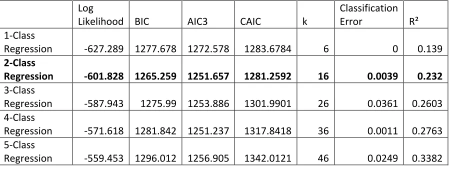
To further explore what exogenous country characteristics help to predict to which growth regime
a country belongs, we then add landlocked, latitude, and settler mortality as covariates. Table 3 presents
the fit statistics for these models. As above, all three information criteria point to the two class model.5 Even with the additional parameters estimated in these models, the two class model with these three
covariates fits the data better than the two class model without the covariates by all measures.
Specifically, this model has improved information criteria, an improved R-squared, and lower
classification error.6
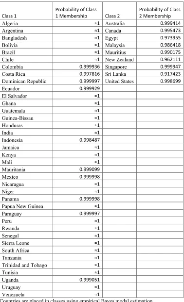
Table 4 displays the class membership for the individual countries in the sample along with the
predicted probabilities of this membership. A couple of points are worth noting. First, certainty of
classification is high for most countries: as can be seen from this table, the majority of countries are in
Class 1 and many countries in Class 2 are placed in their classes with high probability. Second, the
countries in Class 2 do not all share the same observable characteristics such as region or income that are
typically used to group countries. As shown in Table 5, they tend to be faster growing countries, with
lower rates of settler mortality, less likely to be landlocked, and are farther away from the equator. That
said, Class 2 is admittedly small, possibly because use of the settler mortality data restricts our sample,
specifically excluding the European colonizers. We take up this issue with an expanded sample in
subsequent estimations.
The estimated coefficients for the growth regressions and the covariates from this estimation are
displayed in Table 5. In the first column of Table 5, the one-class model is presented and in the second
and third columns, results of the two class model appear. Because class 1 is such a large part of the
5
It is true that the AIC3 for the four class model is very slightly lower than it is for the two class model. However, given that the BIC and the corrected AIC point to the two class model, we justify ignoring this small difference on the basis of parsimony.
6
sample, the one-class model mirrors the results for Class 1 of the two-class model. However, the majority
of the coefficients for Class 2 are statistically different from those of Class 1, suggesting that these
countries follow a different growth process. Specifically, Column 4 of Table 5 reports the p-value of the
Wald tests for the equality of coefficients across classes. These results indicate that except for the
coefficient on investment, all the remaining coefficients for Class 1 and Class 2 are statistically different
from each other. Thus, using the results for the one-class model for these countries could lead to incorrect
conclusions.
In the two-class model, countries are sorted into classes based on a latent variable. What helps to
predict this latent variable? The coefficients that are reported in the bottom half of Table 5 for each
covariate correspond to the gamma parameters in equation 8. These coefficients are reported relative
to Class 1. In other words, a positive coefficient indicates that higher values of the covariate are
associated with greater probability of membership relative to membership to Class 1. The results for the
covariate coefficients suggest that the latent variable sorting countries into different growth regimes is
related to the quality of institutions. Of the three covariates, only settler mortality is significant,
suggesting that institutional quality is responsible for sorting the countries into the classes. Of course,
settler mortality may be affected by geographic features of countries and when we run the model without
settler mortality, the two geography variables have increased statistical significance. Landlocked predicts
membership in Class 2 negatively (at the 1% level) and latitude positively predicts Class 2 membership,
though with lower significance (p-value of .14). The fact that these geography variables no longer are
significant once settler mortality is incorporated into the estimation suggests that geography may play a
role in sorting countries into growth regimes through its effect on institutional development.
Unfortunately, as we mentioned above, although settler mortality has the advantage of being
clearly exogenous, its use excludes countries that were not colonized by Europeans. In order to draw
accurate conclusions about country characteristics that sort countries into classes, the covariates we use
institutions and level of income, it may be justifiable in our context to argue that current institutional
features of the economy are exogenous to the five year growth rates. The arguments in Acemoglu,
Johnson, Robinson and Yared (2008) support our reasoning. They provide evidence that democracy and
income are contemporaneously correlated because they started to develop simultaneously centuries ago.
Therefore, we replace settler mortality with two measures of current institutional quality, democracy and
law and order, allowing us to almost double our sample size.
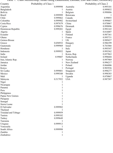
Using the expanded data set, we again estimate models with one to five classes and display the fit
statistics in Table 6. Although in this case the AIC3 indicates a 3-class model, both the BIC and the
corrected AIC suggest a 2-class model. Therefore, we choose the more parsimonious model again and
display the country groupings in Table 7. As before, Class 2 contains faster growing countries, but, also
as before, countries in this group are not all easily classified by the typical region or income groupings.
Importantly, by expanding the sample to include countries that were not colonized by Europeans, we have
added several countries in Class 2. A larger Class 2 emphasizes the importance of allowing heterogeneity
in the growth process because it becomes clearer that there are more than just a few countries who do not
conform to the Class 1 results.
Regression results appear in Table 8. The regression results of Class 1 and Class 2
regression results are different to the one-class model results. In addition, the Wald tests presented in
Column 4 of Table 8 show that both the coefficient on initial income and the coefficient on human capital
are different for both Class 1 and Class 2, suggesting that the effect of increased education and increased
income would be different, depending on which class the country experiencing the change is in. An
examination of the regression results for each class also leads to some interesting conclusions. The
estimated growth regression for Class 1 countries is consistent with a neoclassical, accumulation-driven
growth process. The same conclusion cannot be drawn for Class 2 countries. This regression shows a
positive and significant coefficient on initial income, suggesting a lack of income convergence and the
education, however, suggests that there may be some convergence forces at work as countries with a more
educated labor force grow more slowly.
As before, institutional quality seems to be the most important predictor of class membership,
with law and order being a significant and positive predictor of membership in Class 2. In contrast, the
democracy index is not a significant predictor of class membership. A perusal of the list of Class 2
countries in Table 7 provides insight into this result. Class 2 contains several strong democracies but also
some less-democratic, fast-growing countries too. This result parallels earlier work that found that
political institutions were less important for growth than economic institutions, (e.g. Knack and Keefer,
1995).
In general, our results lend some support to the common practice of treating rich and poor
countries separately, but they also suggest that this practice is far from perfect. Controlling for the
influence of relative backwardness on growth simply by using separate samples of rich and poor countries
fails to take into account significant heterogeneity among countries at similar levels of development.
Although Class 1 contains only developing countries, Class 2 contains both developed and developing
countries. Interestingly, it is the developing countries in Class 1 that feature accumulation-driven growth.
The growth process experienced by the faster-growing Class 2 countries is more difficult to explain with
existing growth theories, except to note that the positive coefficient on initial income is consistent with
these countries being responsible for pushing out the technological frontier.
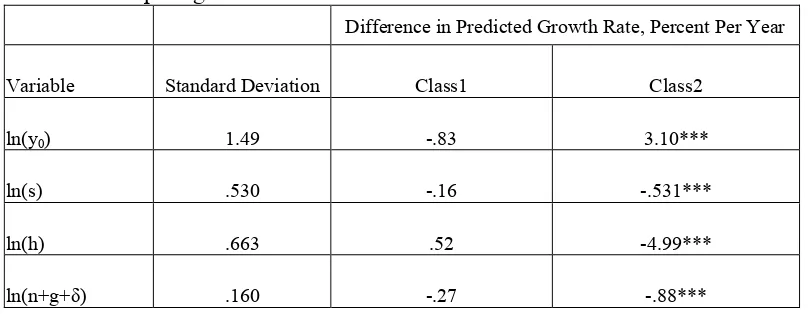
Calculations in Table 9 compare the effects of the coefficients from the two-class model with
those from a standard one-class model. The last two columns of Table 9 show the difference in the
predicted growth effects of a standard deviation increase in each regressor for the two-class and
one-class model. While the differences are smaller and statistically insignificant between the Class 1 results
and the one-class model, these results show that using the standard, one-class approach to make
inferences about Class 2 countries could lead to meaningfully different conclusions.
Although so far our analysis has mainly been descriptive, if we were to infer a causal role for
either the covariates or the regressors in the growth process, the policy conclusions would come at two
levels. First, one type of policy conclusion would address the question: Given the growth process in a
particular country (i.e., the class the country is in), what should be the focus of growth enhancing policy?
For example, investment in education might be recommended for countries in Class 1 but might not
necessarily be a growth priority for countries in Class 2.
Perhaps the more interesting conclusion is the answer to the question, what should a country do to
move to a different group? Countries in Class 1 experience an average growth rate of 1.17. However, the
“typical” country in Class 1 (one that has average values of initial income, investment, human capital and
population growth for Class 1) would grow at 3.81 percent per year if its growth process were described
by the coefficients estimated for Class 2. The disparity in growth rates associated with applying different
estimates of the effects of these growth fundamentals more than explains the difference in growth rates.
Our results then have a clear policy implication for institutional reform that generates greater law and
order in developing countries.
Extensions
Although we use panel data looking at growth over 5-year intervals, our methods can also
theoretically be applied to data that measures growth over longer periods (i.e., cross-section regressions
examining 30 or 40 year growth rates or a shorter panel examining 10-year growth rates). Unfortunately,
the methods are inherently data intensive and finding a parsimonious model that is consistently selected
by all three information criteria with the smaller data sets necessarily generated by these longer term
growth rates is not possible at this time.
We should also point out that, in the results we report, we examine five-year growth rates, but we
constrain countries to be in the same class over the entire period. It is also possible to extend our methods
to allow regime switching (i.e., countries switch classes over the period) via a Markov process. However,
when we estimate models with this switching feature, we are unable to identify a model that fits the data
contrast to that of Paap, Franses and van Dijk (2005) who find instability in the groupings of countries
based on unconditional growth rates. This different result may be due to the fact that we examine the
conditional distribution of growth rates or because of our use of 5 year average growth rates rather than
one-year growth rates. Our covariates, which do not change or change very little over our sample period,
are likely influencing our finding of stability. Nonetheless, such a model also fits well with the
theoretical literature that addresses regime-switching and it is a fruitful area for further research.
4.3 Comparison to standard methods
In the model we presented above, variables proxying for institutional quality and geographic
characteristics were used as covariates to help predict the growth regime to which a country belongs.
This is in contrast to a standard treatment of variables like this in which they are entered separately as
regressors in a one-class model. Before concluding, we also present these standard results and
demonstrate that our methods not only fit the data better, but provide results that have a richer
interpretation.
The results in Table 9 corroborate those found by many others - a negative and significant
coefficient on initial income and a positive and significant coefficient on investment and schooling. The
coefficient on law and order is positive and significant in this regression, but its interpretation is different.
In our method, law and order is not a direct determinant of growth as it is in Table 9, it is a variable that
influences the growth process by helping to sort countries into different growth regimes. Further
comparison of these standard results to the two class model also shows that the two class model fits the
data better in terms of having a lower AIC3, BIC, corrected AIC, and a higher R2, allowing us to confidently reject this standard approach in favor of the two class model.
5 Conclusion
This paper presents a novel application of finite mixture models for estimating growth equations.
Our results suggest that countries follow more than one growth process and that the quality of institutions
these findings is that pooled, one-class analysis that overlooks the heterogeneity in the growth process can
lead to incorrect conclusions about growth in many countries.
The main contribution of our work is to present an empirical technique that matches up with the
theoretical ideas that consider growth to be influenced by both proximate determinants and “deeper
determinants.” In our framework, country characteristics such as quality of institutions influence the
environment in which growth occurs and therefore affect the entire process of growth, determining the
effects of the accumulation of factors of production.
Table 1: Descriptive Statistics
Variable Obs. Mean SD Description Data Source
GROWTH 426 1.75 2.84 Average annual growth
rate over 5 year period
PWT 6.2
Ln(y0) 426 7.85 1.49 Log of initial income PWT 6.2
Ln(s) 426 2.76 .530 Log of investment rate PWT 6.2
Ln(h) 426 1.54 .663 Log of initial average
years of education of labor force
Barro and Lee data set
Ln(n+g+δ) 426 1.89 .160 Log of population
growth + technology growth + depreciation rate
PWT 6.2, g+δ assumed to be .05
Law and Order
426 .621 .240 Index of law and order ICRG
Democracy 426 .676 .212 Index of democracy ICRG
Latitude 426 .296 .192 Absolute value of
latitude
La Porta, Lopez, Shleifer, Vishny (1998)
Landlocked 426 .147 .355 =1 if landlocked Author’s calculations
Settler Mortality
265 4.42 1.10 Log of European settler
mortality
Table 2: Fit Statistics for Model without Covariates
Log
Likelihood
BIC
AIC3
CAIC
k
Clasification Error
R²
1‐Class
Regression
‐627.289
1277.678
1272.578
1283.6784
6
0
0.139
2‐Class
Regression
‐609.505
1269.062
1258.01
1282.0615
13
0.0512
0.2127
3‐Class
Regression
‐600.417
1277.836
1260.833
1297.8362
20
0.0591
0.2363
4‐Class
Regression
‐592.935
1289.825
1266.871
1316.8248
27
0.0976
0.3045
5‐Class [image:23.792.73.522.350.519.2]
Regression
‐583.625
1298.156
1269.251
1332.1558
34
0.0983
0.3484
Table 3: Fit Statistics for Model using Landlocked, Latitude and Settler Mortality as Covariates
Log
Likelihood
BIC
AIC3
CAIC
k
Classification Error
R²
1‐Class
Regression
‐627.289
1277.678
1272.578
1283.6784
6
0
0.139
2‐Class
Regression
‐601.828
1265.259
1251.657
1281.2592
16
0.0039
0.232
3‐Class
Regression
‐587.943
1275.99
1253.886
1301.9901
26
0.0361
0.2603
4‐Class
Regression
‐571.618
1281.842
1251.237
1317.8418
36
0.0011
0.2763
5‐Class
Table 4: Class Membership, Model using Landlocked, Latitude and Settler Mortality Covariates
Class 1
Probability of Class
1 Membership
Class 2
Probability of Class 2 Membership
Algeria ≈1
Australia 0.999414
Argentina ≈1
Canada 0.995473
Bangladesh ≈1
Egypt 0.973955
Bolivia ≈1
Malaysia 0.986418
Brazil ≈1
Mauritius 0.990175
Chile ≈1
New Zealand 0.962111
Colombia 0.999936
Singapore 0.999947
Costa Rica 0.997816
Sri Lanka 0.917423
Dominican Republic 0.999997
United States 0.998699
Ecuador 0.999929
El Salvador ≈1
Ghana ≈1
Guatemala ≈1
Guinea-Bissau ≈1
Honduras ≈1
India ≈1
Indonesia 0.998487
Jamaica ≈1
Kenya ≈1
Mali ≈1
Mauritania 0.999099
Mexico 0.999998
Nicaragua ≈1
Niger ≈1
Panama 0.999998
Papua New Guinea ≈1
Paraguay 0.999997
Peru ≈1
Rwanda ≈1
Senegal ≈1
Sierra Leone ≈1
South Africa ≈1
Tanzania ≈1
Trinidad and Tobago ≈1
Tunisia ≈1
Uganda 0.999051
Uruguay ≈1
Venezuela ≈1
Table 5: Growth regression results for model with covariates
(1) (2) (3) (4) Variable One Class
Model (OLS)
Class 1 Class 2 p-value for Wald statistic for equality of
coefficients across classes Ln(y0) -.7586***
(.2642) -0.8449** (.3202) .079 (0.1548) .01 Ln(s) 2.098*** (.4508) 1.7321*** (.4105) 1.9587*** (0.2209) .63 Ln(h) 1.1240** (.4500) 1.1354** (0.4853) -4.4452*** (0.8854) .00
Ln(n+g+δ) .1383
(1.3673) .2712 (1.3563) -5.5546* (3.2327) .10 Constant -.1106 (2.9179) 0.6645 (3.0398) 15.7242*** (6.5369) .04 Covariates Settler Mortality -2.5781*** (0.8008) Latitude -1.2844 (2.6111) Landlocked -1.2427 (1.095) R2 .14 .10 .61 Class Size
(% of observations)
1.00 .81 .19
Mean Growth Rate
1.23 .84 3.26 Mean Settler
Mortality
4.42 4.81 3.04
Mean Latitude .19 .17 .28 Mean
Landlocked
.12 .15 .00
All estimations include a constant. Robust standard errors are in parentheses. *significant at 10%, **significant at 5%, ***significant at 1%
Table 6: Fit Statistics for model using Latitude, Landlocked, Democracy and Law and Order as Covariates
Log
Likelihood
BIC(LL)
AIC3(LL)
CAIC(LL)
K
Classification
Error
R²
1‐Class Regression
‐1003.95
2033.728
2025.903
2039.728
6
0
0.1882
2-Class
Regression -942.929 1959.026 1936.857 1976.026 17 0.0262 0.3357
3‐Class Regression
‐919.81
1960.133
1923.619
1988.133
28
0.0457
0.3526
4‐Class Regression
‐904.879
1977.617
1926.758
2016.617
39
0.0868
0.4276
Table 7: Class Membership, Model using Landlocked, Latitude, Law and Order, Democracy
Country Probability of Class 1 Probability of Class 2
Argentina 0.999998 Australia 0.995101
Bangladesh 1 Austria 0.999852
Bolivia 1 Belgium 0.998886
Brazil 0.999999 Botswana 1
Chile 0.999862 Canada 0.99893
Colombia 0.999982 Switzerland 0.999687
Costa Rica 0.997679 China 0.870067
Cyprus 0.998676 Denmark 0.999096
Dominican Republic 0.999201 Egypt 0.992165
Algeria 1 Spain 0.816007
Ecuador 1 Finland 0.987361
Ghana 1 France 0.995731
Guinea-Bissau 1 UK 0.989437
Greece 0.694932 Hungary 0.986399
Guatemala 0.999969 Israel 0.761066
Honduras 1 Italy 0.995547
Indonesia 0.999952 Japan 0.993562
India 1 Korea, Rep. 0.857863
Ireland 0.99807 Netherlands 0.998604
Iran, Islamic Rep. 1 Norway 0.997969
Jamaica 1 New Zealand 0.996217
Jordan 1 Poland 0.866006
Kenya 1 Portugal 0.903936
Sri Lanka 0.999801 Singapore 0.998277
Mexico 0.999348 Sweden 0.998383
Mali 1 Uganda 0.870867
Malaysia 0.517952 USA 0.987587
Niger 1
Nicaragua 1
Panama 1
Peru 1
Philippines 1
Papua New Guinea 1
Paraguay 1
Senegal 1
Sierra Leone 1
El Salvador 0.999982
Thailand 1
Trinidad and Tobago 0.999959
Tunisia 0.999182
Turkey 0.999649
Tanzania 1
Uruguay 0.999913
Venezuela 1
South Africa 0.999998
Zambia 1
Table 8: Growth regression Results for expanded sample
(1) (2) (3) (4)
Variable One Class
Model (OLS)
Class 1 Class 2 p-value for
Wald statistic for equality of
coefficients across classes
Ln(y0) -0.5251**
(.2128) -1.0855*** (.2914) 1.5568*** (.2021) .00 Ln(s) 2.4289*** (0.4039) 2.1251*** (0.5845) 1.4337 (1.7876) .75 Ln(h) 0.5015 (.3489) 1.2806*** (0.4439) -7.0309*** (1.7985) .00
Ln(n+g+δ) -1.3215
(1.3002) -2.9622* (1.7682) -6.8274 (8.6135) .66 Constant 7.6721** (3.7793) 11.3477 (14.9745) .80 Covariates Law and Order 10.2372*** (3.3623) Democracy 0.432 (3.0135) Latitude -.0365 (11.0145) Landlocked -0.9167 (1.7812)
R2 .19 .15 .70
Class Size (% of observations)
1.00 .64 .36
Mean Growth Rate
1.75 1.17 2.89
Mean Law and Order
.62 .48 .86
Mean Democracy
.68 .57 .84
Mean Latitude .30 .20 .46
Mean Landlocked
.15 .13 .18
All estimations include a constant. Robust standard errors are in parentheses. *significant at 10%, **significant at 5%, ***significant at 1%
Table 9: Comparing the One-Class and Two-Class Models
Difference in Predicted Growth Rate, Percent Per Year
Variable Standard Deviation Class1 Class2
ln(y0) 1.49 -.83 3.10***
ln(s) .530 -.16 -.531***
ln(h) .663 .52 -4.99***
ln(n+g+δ) .160 -.27 -.88***
Table 9: Standard Growth Regression
Variable
Ln(y0) -1.1864***
(.2611)
Ln(s) 2.3287***
(.4379)
Ln(h) .9647**
(.3822)
Ln(n+g+δ) -1.8598
(1.8074)
Law and Order 3.5284**
(1.4881)
Democracy -1.3443
(1.3292)
Latitude 1.0738
(1.3248)
Landlocked -.8057
(.6735)
BIC 2033.40
CAIC 2043.40
AIC3 2020.36
R2 .22
Class Size
(% of observations)
1.00
References
Acemoglu, Daron, Simon Johnson and James A. Robinson (2001) “The Colonial Origins of Comparative Development: An Empirical Investigation,” American Economic Review 91(5), 1369-1401.
Acemoglu, Daron, Simon Johnson, James A. Robinson, and Pierre Yared (2008) "Income and Democracy" American Economic Review 98(3): 808–42.
Alesina, Alberto and Dani Rodrik (1994) “Distributive Politics and Economic Growth,” Quarterly Journal of Economics 109(2), 465-90.
Alfo, Marco, Giovanni Trovato and Robert J. Waldmann, 2008, “Testing for Country Heterogeneity in Growth Models Using a Finite Mixture Aproach,” Journal of Applied Econometrics 23: 487-514.
Andrews, R.L. and Currim, I.S., 2003, “A comparison of segment retention criteria for finite mixture logit models, Journal of Marketing Research, 40: 235-243.
Azariadis, Costas and John Stachurski, 2005, “Poverty Traps,”
in Philippe Aghion and StevenDurlauf, editors, Handbook of Economic Growth, Elsevier, 295-384.
Benabou, Roland (2000) “Unequal Societies: Income Distribution and the Social Contract,” American Economic Review 90 (1), 96-129.
Bloom, David E., David Canning and Jaypee Sevilla, 2003, “Geography and Poverty Traps,” Journal of Economic Growth 8:355-78.
Bloom, D.E. and J.D. Sachs, 1998, “Geography, Demography and Growth in Africa,” Brookings Papers on Economic Activity 2, 207-95.
Bourguignon, Francios and Thierry Verdier (2000) “Oligarchy, Democracy, Inequality and Growth,”
Journal of Development Economics 62, 285-313.
Boxall, Peter C., and Wiktor .L. Adamowicz, 2002, “Understanding Heterogeneous Preferences in Random Utility Models: The Use of Latent Class Analysis,” Environmental and Resource Economics, 23(4): 421-446.
Canova, Favio, 2004, “Testing for convergence clubs in income per capita: a predictive density approach,” International Economic Review 45(1): 49-77.
Clark, A., F. Etile, F. Postel-Vinay, C. Senik and K. Van der Straeten, 2005, “Heterogeneity in reported well-being: evidence from twelve European countries,” Economic Journal, 115: c118-c132.
Dollar, David and Aart Kraay, 2003, “Institutions, Trade, and Growth,” Journal of Monetary Economics
50(1): 133-62.
Durlauf, Steven N., and Paul A. Johnson, 1995, “Multiple Regimes and Cross-Country Behavior,”
Journal of Applied Econometrics 10, 365-384.
Gallup, J.L, J.D. Sachs, and A.D. Mellinger, 1999, “Geography and Economic Development,”
Greene, William H., and David A. Hensher, 2003, “A Latent Class Model for Discrete Choice Analysis: Contrasts with Mixed Logit,” Transportation Research Part B 37:681-698.
Hausmann, Ricardo, Rodrik, Dani, and Andres Velasco (2005) “Growth Diagnostics,” Manuscript, Harvard University, March 2005.
Knack, Stephen and Philip Keefer, 1995,”Institutions and Economic Performance: Cross-Country Tests Using Alternative Institutional Measures,” Economics and Politics 7(3): 207-227.
Levine, Ross and David Renelt (1992) "A Sensitivity Analysis of Cross-Country Growth Regressions,"
American Economic Review 82(4), pages 942-63.
Mankiw, N. G., D. Romer, and D. Weil, 1992, “A contribution to the empirics of economic growth,” Quarterly Journal of Economics, 107(2): 407-37.
Mauro, Paolo (1995) “Corruption and Growth,” Quarterly Journal of Economics 110(3), 681-712.
Owen A.L. and J. Videras, 2007, “Culture and public goods: The case of religion and the voluntary provision of environmental quality,” Journal of Environmental Economics and Management 54: 162-180.
Paap, R., P.H. Franses, and D. van Dijk, 2005, “Does Africa grow slower than Asia, Latin America and the Middle East? Evidence from a new data-based classification method,” Journal of Development Economics, 77: 553-570.
Papageorgiou, Chris, 2002, “Trade as a threshold variable for multiple regimes,” Economics Letters
77:85-91.
Persson, Torsten and Guido Tabellini (1994) “Is Inequality Harmful for Growth?” American Economic Review 84(3), 600-21.
Rodrik, Dani, Arvind Subramanian, and Francesco Trebbi, 2004, “Institutions Rule: The Primacy of Institutions Over Geography and Integration in Economic Development,” Journal of Economic Growth, 9(2): 131-65.
Sachs, Jeffrey D. and Andrew M. Warner, 1997, “Fundamental Sources of Economic Growth,” American Economic Review 87, 184-88.
Skrondal and Rabe-Hesketh, 2004, Generalized Latent Variable Modeling: Multilevel, Longitudinal, and Structural Equation Models. Chapman & Hall/CRC, Boca Raton, Florida.