On the use of splines in the numerical solution of hyperbolic partial differential equations

On the use of splines in the numerical solution of

hyperbolic partial differential equations.

WISHER, Stephen John.

Available from Sheffield Hallam University Research Archive (SHURA) at:

http://shura.shu.ac.uk/20556/

This document is the author deposited version. You are advised to consult the

publisher's version if you wish to cite from it.

Published version

WISHER, Stephen John. (1977). On the use of splines in the numerical solution of

hyperbolic partial differential equations. Doctoral, Sheffield Hallam University (United

Kingdom)..

Copyright and re-use policy

100250761 8 TELEPEN

SHEFFIELD POLYTECHNIC

Declaration to be signed by each person depositing a thesis

I consent/do not -consent to this thesis being consulted, borrowed or photo-copied.

S ig n e d ; . . VI VVv 1 ... Peflanent address i hJ. ^

St err l-U ^ Lu\a& '...

. ?.‘P..

I, the supervisor, consent/do.not ..consent.

Signed ... ...

Dept,. . . . . ^

Wihout the consent of the author and Cdlege supervisor, no thesis may be consulted, borrowed, or photo-copied for five years after the date of its

ceposit.

De de

I be Si

Pe

I, S: Dc

ProQuest Number: 10701203

All rights reserved

INFORMATION TO ALL USERS

The quality of this reproduction is dependent upon the quality of the copy submitted.

In the unlikely event that the author did not send a com plete manuscript and there are missing pages, these will be noted. Also, if material had to be removed,

a note will indicate the deletion.

uest

ProQuest 10701203

Published by ProQuest LLC(2017). Copyright of the Dissertation is held by the Author.

All rights reserved.

This work is protected against unauthorized copying under Title 17, United States C ode Microform Edition © ProQuest LLC.

ProQuest LLC.

789 East Eisenhower Parkway P.O. Box 1346

O f c

SHEFFIELD POLYTECHNIC LIBRARY SERVICE

ON THE USE OF SPLINES IN THE NUMERICAL

SOLUTION OF HYPERBOLIC PARTIAL DIFFERENTIAL

EQUATIONS

Being a thesis submitted for the degree of

Master of Philosophy

at

Sheffield City Polytechnic

b£

STEPHEN JOHN WISHER

ACKNOWLEDGEMENTS

I would like to express my sincere thanks to my Director of Studies, Dr G F Raggett, of Sheffield City Polytechnic for many helpful discussions during the preparation of this thesis.

My thanks are also due to Dr D F Mayers of Oxford University

for some helpful suggestions on the numerical schemes, to

Dr J A R Stone of Sheffield City Polytechnic for help in deriving

the practical case studies, to the Polytechnic Computer Unit for

the running of my programs and to Mrs Christine Barker for her expert typing of this thesis.

I am also indebted to the Sheffield Education Authority for

the provision of a Research Assistantship.

CONTENTS

Page

Acknowledgements i

Abstract of the thesis it

Chapter 1 - Introduction

1.1 Spline Development 1

1.2 Finite Differences 2

1.3 Present Work 4

Chapter 2 - Spline Functions

2.1 Definition of a Spline Function 6

2.2 Cubic Splines 6

2.3 Multiple Knots 9

2.4 Cubic B-Splines 9

Chapter 3 - Hyperbolic Partial Differential Equations with Constant Coefficients

3.1 Simple Initial and Boundary Conditions 11 3.2 Cubic Spline Finite Difference Scheme 11

3.3 Truncation Error 17

3.4 Stability Analysis 19

3.5 Comparison with a well known Finite Difference Scheme 22 3.6 Truncation Error and Stability Conditions for (3.5.2) 23

3.7 Numerical Procedure 25

3.8 Evaluation of Truncation Errors 29

Page Chapter 4 - Hyperbolic Partial Differential Equations

with Variable Coefficients

4.1 Cubic Spline Finite Difference Scheme 33 4.2 Truncation Error and Stability Conditions for (4.1.6) 37

4.3 Comparable Finite Difference Scheme 41 4.4 Truncation Error and Stability Conditions for (4.3.2) 43

4.5 Numerical Procedure and Evaluation of Truncation

Errors 46

4.6 Singularities in the Variable Coefficients 48

Chapter 5 - Unequal Step Lengths

5.1 General Considerations 49

5.2 Cubic Spline Finite Difference Approximation to

(3.1.1) 51

5.3 Finite Difference Approximations to (3.1.1) 59 5.4 Truncation Errors and Stability Conditions 61 5.5 Difference Schemes with variable ©( and Q 63

5.6 Equations with Variable Coefficients 65

Chapter 6 - Case Studies

6.1 Case Study 1 68

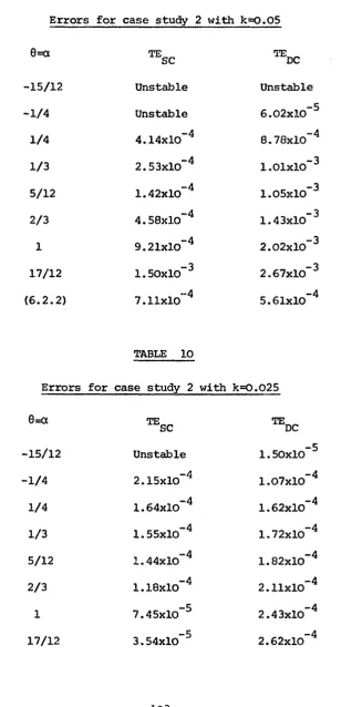
6.2 Case Study 2 77

6.3 Case Study 3 79

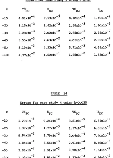
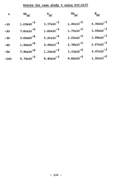
6.4 Case Study 4 83

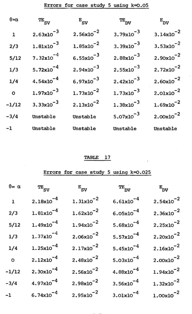
6.5 Case Study 5 84

Chapter 7 ~ Conclusions and Extensions

Conclusions 90

Extensions 97

Tables and Figures 99

Appendix 109

CHAPTER 1

Introduction

1*1 Spline Development

A spline is a simple mechanical device used by draftsmen for drawing smooth curves. It consists of a slender bar made of wood or some other flexible material to which weights are attached. The spline is placed on a sheet of graph paper and constrained by use of the weights so that it takes the shape of the curve we wish to draw. The term "spline function" was first used by Schoenberg (1946) in a paper describing the use of generalised splines and other piece-wise polynomials to approximate smooth functions of one variable. The properties of spline functions were in fact employed in a few isolated instances before this date although no reference was made to the name itself. Schoenberg's early paper was an important con­ tribution to the use of spline functions but it was not until the 1960's that further work in the field was published.

In recent years spline functions have been used to solve a wide range of numerical problems. For example Birkhoff and De Boor

(1965), Curtis and Powell (1967) and Schumaker (1969) have described methods of interpolating and approximating functions whilst the numerical solution of ordinary differential equations has been con­ sidered by Bickley (1968), Fyfe (1969) and Albasiny and Hoskins (1969), Although El Tom (1974, 1976) has proposed several spline function

moving boundary problems in heat flow was discussed by Crank and Gupta (1972), In their paper the authors used the spline function not to obtain general solutions to the problem but to determine the position of the boundary at each time level.

The general numerical solution of the well known one-dimensional heat conduction equation was considered by Papamichael and Whiteman

(1973)• A similar method has since been used by Raggett and Wilson (1974) to obtain solutions to the one-dimensional wave equation. These last two papers form the basis of the work described in this thesis.

*•2 Finite Differences

As will be seen in the following chapters we compare our methods using cubic splines with a well known fully implicit finite difference approximation. It is therefore useful for us to briefly describe the development of finite difference methods for the numerical solu­ tion of partial differential equations.

by von Neumann for the numerical solution of the wave equation.

Since von Neumann’s work on finite differences there have been many types of schemes proposed, possibly the most well known being that of Crank and Nicolson (1947). The majority of these schemes use

rectangular grids which have constant step lengths in both the time

and space directions. There are, in fact, very few instances where unequal step lengths have been used for solving partial differential

equations. Murray and Landis (1959) deformed the grid in the space direction by compressing or stretching it as an aid to solving

moving boundary problems in heat flow. They considered the problem where the boundary between a solid region and a liquid region is moving with time. They then approximated the heat conduction equa­

tion, which describes these practical circumstances, by finite difference approximations with a constant step length on the solid

side of the boundary and a different constant step length on the liquid side. This meant a change in the size of the step length from one side of the boundary to the other.

Moving boundary problems of this type are often referred to as "Stefan problems" and have also been solved using an alternative

variable step length method due to Douglas and Gallie (1955). In this paper the authors introduced a variable time step length while

keeping the size of the space mesh length fixed. This method is particularly useful in solving parabolic equations where, with the increase of time, the solution becomes smoother and smoother. It

is therefore advisable to use a small time step length at the

1.3 Present Work

As suggested in section 1.1 a great number of numerical

problems can now be solved with the aid of spline functions. In

chapter 2 we define spline functions in general and derive some expressions which results from the definition of the cubic spline, this being the degree of spline function we will use throughout this thesis. The cubic spline definition and these resulting

expressions are given in detail in Ahlberg, Nilson and Walsh (1967).

It was indicated by Raggett (1974) that the cubic spline method for solving the one-dimensional wave equation (see Raggett and Wilson (1974)) could be extended to obtain solutions to more general hyperbolic partial differential equations. This work is

shown in chapter 3 where, in addition to the splines schemes, we have derived a well known implicit finite difference approximation from which we will draw comparisons.

In chapter 4 both the splines scheme and the difference approxi­ mation are developed to cover equations having variable coefficients. The methods of solution in both this chapter and the previous one

require the Knots for the splines schemes and the mesh points for the difference schemes to be equally spaced. The extension of the

r

methods to cover arbitarily spaced knots and mesh points is given in chapter 5.

The truncation errors and stability analysis for each of the constant coefficient and variable coefficient schemes, both using constant step lengths and variable step lengths, are given in their

respective chapters. Numerical procedures are also described for

These additional solutions are found directly from the spline func­

tion itself. This is found to be a major advantage of the splines

schemes over the more well known finite difference methods. In chapter 6 several case studies are developed where equa­

CHAPTER 2

Spline Functions

2.1 Definition of a spline function

Consider an interval a £ x £ b and subdivide it into m sub-

intervals by inserting knots at the points x^, x^, ... , where

a = x < X. < ... < x = b _{o 1 m} (2.1.1)

Then a spline function s(x) of degree n with knots x , x,, ... , x_{o 1 m} is a function possessing the following two properties.

(i) In each interval x^ ^ £ x £ x^ (i = 1,2, ..., m) , s(x) is a polynomial of degree n or less.

(ii) S(x) and its derivatives of orders 1,2, ..., n-1 are con­ tinuous .

Thus a spline function is a piece-wise polynomial function satis­ fying certain conditions regarding continuity of the function and its derivatives. As explained by Greville (1969) when n = o condi­ tion (ii) is not operative and a spline function of degree 0 is a

step function. For n>0, a spline function of degree n could th

equally well be defined as a function whose n derivative is a step function.

2.2 Cubic Splines

Let f(x) be a function with continuous derivatives in the range a( x < b. Then Six) is a cubic spline interpolating to the func­ tion f(x) at the knots x , x , ... r x_{o 1 m} if

(ii) S'(x) and S"(x) are continuous

(iii) S(x.) - f(x.) (i = _{1 1} 0,1, ... , m).

Thus a cubic spline consists of a set of cubic polynomial arcs

joined smoothly end to end. The smoothness consists of continuity

up to the second derivative, but the third derivative will, in general, have a discontinuity at each of the points x = x.

(x — 0, 1, ... , m)«

If we represent S"(xj, the second derivative of the cubic spline at the points x = x^, by M then from Ahlberg, Nilson and Walsh (1967) we have from the linearity of the second deriva­

tive on the interval x. ., x.

L

i-1

i J

S"(x) = M. , / X. - X \ + M. / x - x. , \ (2.2.1)

i-1' _i

1

I

izi 1

V hi

)

\

hi

j

where h^ = x^ - x^ Integrating twice and evaluating the constants

of integration, we obtain

S (x) = M. . (x. - x) _{x-1 x_____} 3 + M. (x - x. ) _{x _____ x—1} 3 + / _! f (x. .) - h_{x-1 _x_ i-l I}.2 M. \

6h . 6h, ■ 6 j

i i

(x. - x) + / f(x.) - h._{l [ l i i ’}2M.\(x - x. ) (i » 1,2, ...,m)

(2.2.2)

S’ (x) = -M. i (x. - x) + M. (x - x. .)'•* + f(x.) - f(x. ,) _{l-l i x i-l l i-l}

2h. _x 2h. _i h ._i

M. - M. . \h. _{x i-l i i} (i = 1,2, ... ,m) (2.2.3)

From (2.2.3) we have the expressions for the one-sided limits of

S'(x. -) = h. M. . + h. M, + f(x.) - f(x, .) (i = 1,2, ..., m) _{l i i-l 1 1 l i-l} h.l

(2.2.4)

S'<x± +) = -h.+1 M. - hi+1 Mi+X + f(x1+1)-f(x.) (i = 0,1...

3 6 hi+l

(m-1)) (2.2.5)

From the continuity of S *(x) at the points x = x^ (i * 0,1, ..., m)

we can equate (2.2.4) and (2.2.5) thereby obtaining the expression

hi Mi-i + ,/hi + hi+i',Mi + hi+i Mi+i = f(*i+i) - f(xi> - f(xi) - f(xi-i)

6 V 3 j6 hi+1 ht

(i = 1,2, ..., (m-1)) (2.2.6)

Given the function values f(xj (i = 0,1, ...,m) we require two additional conditions in order to express (2.2.6) in tri-diagonal

form. As shown by Curtis (1970) there are three choices available for these two extra conditions, namely

(i) S"(x±) — 0 (i = 0,m) (2.2.7) (ii) S'(x.) = f'(x.) (i = 0,m) _{i l} (2.2.8)

(lil) [sex) - f<x)]x=l5(x^ i+Xi)=[s(x) - f(*)]x=!s(Xi+Xi+i)

(i = 1, m-1) (2.2.9)

Each of these conditions can easily be applied in practice although the second used by Birkhoff and de Boor (1965), and the third,

Once the choice of "end conditions" has been decided upon, substitution of these into (2.2.6) gives a system of (m-1) equa­

tions which are linearly independent, tri-diagonal and diagonally dominant. They can therefore easily be solved for the values M. (i = _i 1,2, ...,(m-1)), the satisfaction of the "end conditions”

then giving Mq and M^. The spline function S(x) can then be

obtained from (2.2.2). 2.3 Multiple Knots

The condition (2.1.1) can be relaxed to the form (see for

example Cox (1975))

a = x < x, _{os: 1} ... < x = b _{s m} (2.3.1)

If in general the points x^ to are such that

x = x _{r r+1} = ... = x _r+k-1 = x _r+k (2.3.2)

then these coincident knots can be regarded as a single knot of

multiplicity k* In a case such as this the spline function S(x) of degree n has n - k - 1 continuous derivatives instead of the

original n -1 as stated in section 2.1. For example, at a knot of multiplicity 2 the cubic spline function is itself continuous

but has no continuous derivatives. Similarly, for a cubic spline which has a multiple knot of degree 3, the function S(x) has a

jump discontinuity and it is therefore of no use to consider knots

of multiplicity which are greater than the degree of the spline function itself.

2.4 Cubic 3-Splines

equally spaced knots, was first introduced by Schoenberg (1946).

These B-splines can be shown to be non-zero only over a small

number of intervals between successive knots.

For the particular case of the cubic B-spline we can define

this as being a cubic spline which is zero everywhere except over four adjacent intervals between knots. Using the notation

employed in section 2.2 this means that the cubic spline function with knots x. _{*4 JL}x. , x. , x. and x. is zero everywhere in_{mmm o i—x X}

the range a x b except within the interval < x x^.

These cubic B-splines have been shown to be useful for fitting

CHAPTER 3

Hyperbolic Partial Differential Equations with Constant Coefficients

3.1 Simple Initial and Boundary Conditions

Suppose that u(x,t) satisfies the second order hyperbolic partial differential equation

32u = a 32u + b 3u + cu (0 £ x £ 1, t >0) (3.1.1) 3t2 3x2 8x

where a,b,c are constants and a>0. We consider (3.1.1) to be subject to the following boundary conditions

u(0, t) = fL(t) ; u (1^ t) = f2(t) (3.1.2)

and initial conditions

u(x,0) = g (x) ? 3u (x,0) = g9(x) (3.1.3)

1 3t

where f (t) , f2(t), g^x) and g2 (x) are known functions. These conditions are only of a simple form but, as is shown in section

3.9, they can be of a more general nature and the following methods of solution will still apply.

3. 2 Cubic Spline Finite Difference Scheme

To obtain solutions to (3.1.1) we will initially consider the interval 0 £ x £ 1 subdivided by equally spaced knots where the step length between successive knots is h, so that x^ = ih

U . _ - 2U. + U _{i/j-1 i/j i/3+l} - = a / 0M. , . + (1-20)M. . + 0M._{| i/j-1 1/3 i/3+1}

k2

+ b | 0L. . _ + (1-20)L . . + 0L. \ J i/3-l 1/3 i/3+lf

+ c < 0U . + (1-20)0. . + 0U. ..._{i/3-l i/3 i/j+1}

(3.2.1)

(i = 0,1, ... , N ; j = 1,2, ... ; Nh = 1)

where L, . = S’ (x.) M. . = S'! (x.) ; S . (x) denoting the cubic i/3 3 1 i/3 3 1 3

th

spline interpolating the values U. .on the j time level. 1/3

With constant step length h the spline function (2.2.2), for

th r -i

the j time line within the interval x. ,, x. j , becomes

L

i“1

1

J

S.(x) = M . (x.-x)3+M. . (x-x .)

3

+/u.

6h 6h 6 h

+ /U. . - h2 M. . \ (x-x. .) (i = 1,2,...,N) (3.2.2) { ±t3 6“ 1 0 J

----4 » rst

and thus the continuity of the oooond- derivative of the cubic spline

with equally spaced knots on the j time line gives

1 M. . + 2 M. . + 1 M .. . * U. , - 2U. . + U . . (3.2.3) ^ 1-1,3 j _1,3 6 _1+1,3 i-l,j 1,3 1+1/3

h2

(i = .... (N-l)) th

This equation also holds on the (j—1) time line

1 M + 2 M. + 1 M . = U, _ . - 2U. . _ + U. . . . g i-l,j-1 y l/j-l y i+l,3-l i-l,3-1 i/j-1 1+1,j-1

th

and on the (j+1) time line

1 M. . + 2 M . + 1 M. _ = U. . - 2U. , . + U4J,

y 1-1,3+1 y i, 3+1 y i+l, 3+1 i-l, 3+1____ 1,3+1 i+l,3+1 h 2

(i = 1,2, ...,(N-1)) (3.2.5)

We now wish to form a relationship similar to (3.2.3) incorporating

the first derivative of the cubic spline. Writing L. . = s' (x.), i,3 j i then (2.2.4) and (2.2.5) respectively become, on the time line

L. . = S', (x.-) = h M. . . + h M. . + U. . - U. _ . i»3 3 i 7 1-1/3 y i»3 1/3 1-1/3

6 3

h---(i = 1,2, ...,N) (3.2.6)

L. . = S'. (x.+) = - h M . - h M _{1/3 3 i y i,j y 1+1,3} . + U.A. . - U. _{1+1/3 1/3}

(i = 0,1,..., (N-l)) (3.2.7) From (3.2.6) we have

L . _ . = h M. . + h M. .. . + u. . . - U._{1+1,3 g 1/3 y 1+1/3 i+l / 3 i/3} h

(i = 0,1, ..., (N-l)) (3.2.8) and from (3.2.7)

L. , * - h M. . , - h M. . + U. _{1-1,3 y i-l, j y i,3 1/3} . - U. . ._i-1/3

h

(i = 1,2, ..., N) (3.2.9)

To obtain the required relationship, equations (3.2.6) and (3.2.7)

are now added together and the result added to half the sum of th

1 L, . . + 2 L, . + 1 L. . • - U_- . - U. . . (3.2.10) g i-l, 3 j if j g i+lrl i+l, j x-1,3

2h

(i = 1,2, ..., (N-l))

As with the expression for the ^ values, (3.2.10) also holds on f*V\

the (j-1) time line

1 L. . . _ + 2 L. . . + 1 L _ . . » IT . . n - U. . . . g- i-l,3-1 -j 1,3-1 g i+l, 3-1 i+l,3-1 i-l,3-1

2h

(i = 1,2, ..., (N-l)) (3.2.11) and on the (j+1)^ time line

I Li-1,j+1 + | Li,j+1 + | ^i+1,j+1 “ Ui+l,j+l ~ Ui-1,j+1 2h

(i = 1,2, ..., (N-l)) (3.2.12)

To obtain the finite difference scheme incorporating splines we now combine the above relationships for the M. . and L._{1/j if j} values by performing the following

operations:-(i) Equation (3.2.3) is multiplied throughout by a(l-20)

(ii) Equations (3.2.4) and (3.2.5) are summed and the resulting equation is multiplied throughout by a0.

(iii) Equation (3.2.10) is multiplied throughout by b(l-20)

(iv) Equations (3.2.11) and (3.2.12) are summed and the resulting equation is multiplied throughout by b0.

-a (1-20) / 1 M. , , + 2 H, . + 1 M. . . \

\6

1,3 6 1+1,3

j

+ a6ii Mi-1,j-1 +

f

+ i “ifl, j+1 )

+ b (1-20) / 1 L. . + 2 L. . + 1 L . . \ { _{6 3 X'j 6 i+1'3} I

+ b0[ 1 L. _{^ - x-1,3-1}. - + 2 L. . . + 1 L . . . _ + 1 L . _ _{-j x,3-1 ^ i+l,3-1 - x-1,3+I j x,}+ 2 L. _3+I

+ | Li+l,j+l

- a(1-29) ' ui-i,i - 20i , j+ V 1.1 ^

h2 J

+ a0 / U. , . . - 2U. . . + U. _ . . + U. , _{i-l/3“l x ,j—1 x+1,3-1 x-1,3+I} - 2U. _x,3+I + U. _{x+1,3+1 j}\

h2 h2 1

+ b (1-20) / U. _{( J-+1/3} . - U. _ . \ + b0/ U. _{x-1,3 J j i+l, 3-I} . - U. . . ._x-1,3-I

V 2h 7 \ 2h

* Ui+1,j+1 ~ Ui-1,j+1 ) (3.2c13)

2h

We now eliminate the M.. and L. . values from the left hand

13 i,3

side of (3.2.13) using (3.2.1). The following three time level finite difference scheme incorporating splines then results,

(1-3 0)U. . ... _{1 x-1,3+1} + 4(1+0 _{2 x,}9)U. ₃... + (1-0 0)U_{+l 3 x+1,3+1}

= {2 + 0 (l-20)}u. . , + 4{2-0_(l-20)}u. . + _{1 x-X,3 l x,3} {2+0-(1-20)₃ }u. _ ._i+l,3

- (i-e.e)u _{1 x-1,3-1} - 4d+e_e)u. . . - u-e,e)u_, . , _{2 i,3~1 3 x+1,3-1} (3.2.14)

where 0, = ₁ 6ar - 3brk +ck ; 0„ = 3ar - ck ? 0_ - _{* j} 6ar + 3brk + ck‘

and the mesh ratio r = k/h.

This difference scheme is implicit in nature and has three unknown values on the advanced time line t = (j+l)k. It can there­

fore be expressed in the form of a tridiagonal system of equations and solved using an algorithm based on the Gaussian elimination

process. We will describe the solution of these tri-diagonal systems in the Twrtwir appendix:**.

3.3 Truncation Error

To obtain the truncation error associated with (3.2.14) we

first rearrange the scheme into the form

(1-619) (Ui-l,j+l + V l . j -11 + 4 U + 626) (Ui,j+l + 0₁. . .)_13“l

+ (1 - 0-0) ₃ (U. _i+l,j+1 + U _i+l,3. )_-I

(2 + 0 (1-20)>U. . . + 4(2 - 0-(1-20)>U._{1 i”l(j 2 i,j}

+ {2 + 0_(1-20)>U _{3 1+1,3}.

(3.3.1)

We now expand each term of (3.3.1) about the mesh point (ih,jk) using Taylor series approximations. The following expression,

+ 4(l+020) 2U. . + k2 t 32u \ + k* / 3*u U t 2 /. . 12U t V . .

1,3 i,3 “

+ d-e30)

lu.

\

\

* /

\

I 1'

\3x /i,j 2f U x 2 /. . 3I\3x3/. . 4*V3xV.

+k21/ 32u \ + h / 33u 3t2/ . ^3x3t2

i,3 1,3

+ h2 / #>«» a u

21 ' 3x23t2

1

. J

12

I

i,3 i,3

* {2+31(1-26)> U. hi 3u_\ + h/^ / 32u \ - h_^ / 93u \ + h^_ / 3*u } 1,3 '3x/i,j

21 U 2/

3!-l

I

i,3 i,3 i.

+ 4{2—3_(_Z 1-20)} U, ._{, J}

+{2+ ^ (1-20)} U. h/3u \ + h2/ 32u \ + h3/ 33u \ + h* / 3*u \

1,3 2' U A . 3!U x 2 / . 4 : U W . .

i,3 i,3 i,3

(3.3.2)

we obtain the following truncation error for (3.2.14)

k2h2Ic2r2f(0)u + 2bcr2f(6) 3u

I 3x

+ ) r2(2ac + b2)f(0) - 1 c2k20 i 3fu

i

i

2abr f(0) - _1 bck 0i3“u

6 ■2a|

,

>-j a x3

+/a2r2f(0) + 1__ a - 1_ ch2- 1_ ack20{ _{a u}

12 72 6 f dx* (3.3.3)

where f(0) = 1_ (1 - ck 0) - 0

12 (3.3.4)

3.4 Stability Analysis

To examine the stability of (3.2.14) we use the well known von Neumann method. Initially we replace U. , by U _{i i J m,n} in (3.2.14)

so as to avoid any conflict between variables and then look at solutions of (3.2.14) which have the form (see Mitchell (1969))

0_m„n = eim^ einX U2 = ■1) (3.4.1)

where Y is an arbitrary real number and

X

to be determined. Substituting (3.4.1) into (3.2.14) and dividing by e^‘mYe'*'nA, we obtain

Due to the expressions

2Cos A = e + e

and

A = 1 - 2Sin2A^

2

we can replace (eiA+e iA) in terms of Sin2

A

2(l-2Sin2A)

j

= {2+3x(1-20)}e"lY+4{2-32(1-20)} + {2+33(1-20)}elY

(3.4.2)

If we now replace the factors 3^, 32 and 33 by their full expressions

as given in (3.2.14) and let h and k tend to zero in such a way as r remains fixed then we obtain

Sin2

A_

2 3-2(l-6ar26)Sin2y/2

For stability we require n to be bounded. Therefore

A

O * Sin2

A

2

must be satisfied. Substituting (3.4.3) into (3.4.4) and noting that Sin2y/2 £[0,l] we have

Hence the following conditions governing the stability of (3.2.14) are obtained

(a) if 0 Z h _{it is unconditionally stable}

(b) if 0 < \ it is stable when

r * (3a(1-40)J”*2 . (3.4.5)

It should be noted that the stability condition (3.4.5) does

not depend on the coefficients b or c. Fox (1962) indicated that when solving the general parabolic partial differential equation

3u = a 32u + b 3u + cu + d (3.4.6) 3xJ

oTt ^ 2 3x

where a, b, c and d are functions of x and t only, then it is reasonable to assume that the presence of the lower order terms, u and 3u/3x, have no great effect on the stability condition for

a particular finite difference scheme. This assumption is borne out in two examples given by Richtmyer and Morton (1967). In the

hyperbolic equation (3.1.1) it appears that this conjecture is also true since the quantities u and 3u/3x are also effectively multiplied by h and h respectively as was the case in parabolic

equations. However, although the stability condition is practically

unaffected by these lower order terms, it must be noted that they may require a smaller value of k to be used. For example (see Richtmyer and Morton (1967), page 195) if a large value of c is

3.5 Comparison with a well known finite difference scheme

As a comparison to the method incorporating cubic splines, which was derived in section 3.2, we now consider the well known

implicit finite difference scheme as an approximation to (3.1.1). This method was described by Mitchell (1969) for the solution of the wave equation and is easily extended to our more general case, giving at (ih,jk)

(i » 1,2, ..., (N-l) ; j = 1,2, ... ; Nh = 1)

where r = k/h. Rearranging this into a form similar to (3.2.14) we have

U. . .-2u. ,+u. 1,3-1 1,3 1,3+1

r

+(l-2a)(u

+(l-2a)(ui.., .-u. _ . _{1+1,3 1-1,3}

+ck2{au. . .+(l-2a)u. .+au.

i,3-l i,3 i,3+l (3.5.1)

= jfar2-bhr2 l(l-2ot)lu, , .+ {2+(-2ar2+ck2) (l-2ct) } u,

+ J *'ar2+ bhr2 ) (l-2a) i u. . .

} ■ ~2— 1 '3

-ot'-ar2+bhr2 \ u. , . ,-{l+ot(2ar2-ck2)} u. . ,-a/-ar2-bhr2\ u. ,, , ~2— ' '3 x»3-l 1 ~2— I i+l, 3“1

(i = 1,2, ..., (N-l)). (3.5.2)

The choice of a=0 in (3.5.2) gives rise to the usual explicit

approximation to (3.1.1). Also, as shown by Raggett and Wilson

(1974), when solving the wave equation (a=l, b=c=0 in (3.1.1)) the approximation (3.2.14) reduces to (3.5.2) when 0 =01 + 1

6r2

3.6 Truncation Error and Stability conditions for (3.5.2)

The truncation error for the scheme (3.5.2) is obtained in

the same manner as that of (3.3.3) and is seen to be, at (ih,jk)

k2h2; c2r2f(ot)u + 2bcr2f(ot) ^u + r2 (2ac + b2)f(ot) S2u

| 9x

r j f

+ i

1

6 j

I

12 j

j

where the function f~is given by (3.3.4)

The nature of the two truncation errors (3.3.3) and (3.6.1)

are very similar, there being a number of like terms when the parameters ot and 0 are chosen equal. The two truncation errors

2 2

are 0(k h ) and both may be considerably simplified by choosing the function f to equal zero. Thus from (3.3.4), 0 and a are

Sx"

chosen such that

6 = a = 1 (3.6.2)

12 + ck2

Methods of choosing a and 6 in order to increase the accuracy of the two schemes will be discussed in the later chapter covering case studies.

A detailed von Neumann stability analysis of the scheme (3.5.2) gives the following conditions for stability:

(a) if ot ^ k it is unconditionally stable (b) if a < h it is stable when

r * {a(l-4a)}”S5 . (3.6.3)

In view of the fact that the two truncation errors (3.3.4)

and (3.6.1) are of the same order and that the stability condi­ tions are very alike for both schemes (3.2.14) and (3.5.2), then

both schemes seem equally viable for obtaining the solution to (3.1.1). Both schemes are three time level and require the evalua­ tion of a tri-diagonal system of equations. It is therefore accept­

able to assume that the computing times for both schemes will be very comparable. Relative advantages of the two methods will be discussed in the later case studies although it is clear that sun

additional advantage of using the cubic spline scheme is that it is possible to obtain a spline function from (3.2.2). This can then be used to obtain solutions at points intermediate to the

mesh points on any particular time line. The procedure for

obtaining these intermediate solutions is included in the following

3.7 Numerical Procedure

The method for obtaining cubic spline solutions at points

intermediate to mesh points is similar to that given by Raggett and Wilson (1974) for solving the wave equation. However for the general hyperbolic partial differential equation (3.1.1), the procedure is considerably more complicated by the presence of the L. ,'s in (3.2.1). The steps in the numerical procedure

1r ₃ are as follows:

(i) Evaluation of the M. _i,o , i - 0,1, ..., N.

Using the function value initial condition given in (3.1.3)

equation (3.2.3) with j = 0 gives

which is a tri-diagonal system with (N-l) equations and (N+l) unknowns. As indicated in section 2.2 we require two "end condi­

tions" in order to obtain the M. values from (3.7.1). These_i,o additional conditions are found by putting 6 = j = 0 in (3.2.1) and by making use of central difference approximations to represent the derivative initial condition in (3.1.3). Thus on the boundaries x = 0 and x = 1 we have

(3.7.1)

(i = 1,2, .., (N-l))

(3.7.2)

k2(all +bL ) = _{N f O N f O} 2(f,<k)-f,<_{m ^} 0)-kg,<l>)-ck2f_(0). (3.7.3)

Similarly, from (3.2.7)

L _0,0 = - h M _{— o,o ~ l,o} - h M, + g,(h)-g,(O) _{1 1} (3.7.4)

and from (3.2.6)

Ln,o = ^ mn.o + t V i , o + gi (1>-gi (V i ) (3’7 ‘5)

3 6

h---Equations (3.7.1) - (3.7.5) are (N+3) in number and are solvable

for M. _i,o , i = O, 1, ..., N along with L _{* o,o} and L ._N,o

(ii) Evaluation of the L. _1,0 , i = 1,2, ..., (N-l)

Averaging (3.2.6) and (3.2.7) gives

L. = h (M. . . - M. . .) + U4J- . - U. . . _{i,j i+l» 3 i+1,3 i-l,3} (3.7.6)

2h

(i = 1,2, ..., (N-l))

Having obtained M. _1,0 (i = 0,1, ...,N) in the previous step, we

now put j = 0 in (3.7.6) giving the required values of the 0 's*

(iii) Cubic Spline solution on the initial time line.

Using the fb Q values found in step (i) equation (3.2.2) is used directly to evaluate spline solutions at any point on t = O.

(iv) Mesh point solutions on time line t = k.

gives the set of (N-l) equations

2U -ei6)Ui-l,l + 8(1+629)ul,l + 2(1-639)ui+l,l

= {2 + ei(l-2e)}g1(xi_15 + 4{2-e2(l-20)}g1(x±)

+ {2+63(X-20)}g1(xi+1) + 2k(l-610)g2 (xi_1)

+ 8k(l-826)g2(x1) + 2k(l-830)g2 (x1+1) . (3.7.7)

(i = 1,2, ...,(N-l))

Since uq ^ = f^(k) and ^ 2. = ^ 2 ^ the*1 these with (3.7.7) give an easily solvable tri-diagonal system for the unknown mesh points values u. -, i = 1,2, ...,(N-l)._{X , X}

(v) Evaluation of the M. _1,11 , 1 - 0 , 1 , ..., N.

These values are evaluated in a similar manner to the correspon­ ding M _1,0 values found in step (i). From (3.2.3) with j = 1 we have

1 M. . .+ 2 M. _ + 1 M. = u. . . -2u. _ +u. . , (3.7.8)

-p-_o i-1,1 -r- ₃ 1,1 — ₆ 1+1,1 _---1-1,1 1,1 1+1,1

h2

(1 = 1,2, ...,(N-1))

As in step (i) we require additional conditions in order to obtain the required values. These are obtained in a similar manner, giving the following results

k2(aMN x+bLN x) = f2(0)-2f2(k)+f2 (2k)-ck2f2(k) (3.7.10)

(3.7.11)

h

(3.7.12)

h

Again we have (N+3) equations which are solved for MX f X (i = 0,1, ...,N), L _{O f x} . and L ..._{JM / JL}

(vi) Evaluation of the Li/1 i = 1,2 • / (N-l) .

These values are evaluated in a similar manner to the

correspond-used with j = 1, the x values required being known from step (v).

(vii) Cubic spline solution on t = k.

As in step (iii) equation (3.2.2) is used directly, with j = 1

in this case.

(viii) The General scheme.

A full spline solution over two successive time lines is now known. Suppose the scheme is fully developed and that solutions are known along the (j-l)^ and 3 th time lines. Then equation

(3.2.14) along with the boundary conditions (3.1.2) constitute

a tri-diagonal system of linear equations which is solvable for the mesh point values u. ._1,3+1 i = 1,2, ...,(N-l).

M. . . , i =0,1, ..., N (3.2.1) gives (N+l) equations in the 1 / J“

J-2(N+l) unknowns L. _{1,3+1 1,3+1} i = 0,1, ...,N. A further two

equations are obtained from (3.2.7) with i = 0 and from (3.2.6) with i = N. The remaining (N-l) equations are obtained from (3.7.6)

th

now evaluated at the (j+l) time line. Equation (3.2.2) then give any required intermediate values on this new time line.

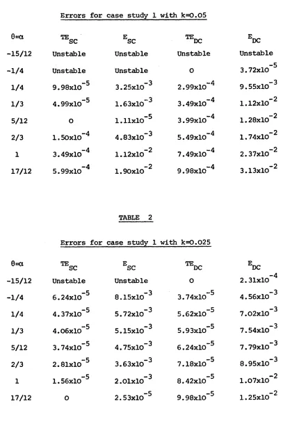
3*8 Evaluation of Truncation Errors

To estimate the accuracies of the finite difference formulae

(3.2.14) and (3.5.2) we will obtain numerical values of their respective truncation errors. The derivative terms within the truncation errors are evaluated using relevant forward and backward difference approximations on the boundaries and central difference approximations for the internal mesh points. For example

S^u \ - 1 (U. _{— i+2,j i+l,3} -4U. . .+6U. -4U. . .+U _ .) _{i/j 1-1/3 1-2,3} (3.8.1) \ Sx** /. . h**

1/3

and using mean central differences, to avoid having to evaluate

solutions at half-way points between mesh points, we have

93u \ = 1 (U. .-2U. . .+2U. . ,-U. _ .). (3.8.2) — 7 — 7 1+2'3 1+1'3 1-1'3 1-213

3x /. , 2h i/j

3.9 Derivative Boundary Conditions

The boundary conditions given in (3.1.2) can be generalised to the form

a3(t)u(l,t) + a4(t) 3u (l,t) *= f2 (t) (3.9.2) 3x

where a^(t), o^Ct), a^(t) , a4 (t), f^ft), are known functions

which are continuous and bounded as t ■+ The implementation of (3.9.1) and (3.9.2) is reasonably simple and, for convenience, we will illustrate the procedure for (3.9.1) only. It is usual to represent the derivative in (3.9.1) by the central difference approximation giving (see for example Fox (1962) p 248)

a (t)U _{1 0,3} + a (t) / U. . - u .\ = f, (t) . _{2 / 1,3 -1/3} (3.9.3)

Rearranging to make U ^ the subject of the equation we have

U , . = U, , - 2h / f,(t) - a n (t)U_ , ) (3.9.4)

_1'j llj S^TtT \

1

1

°'3

I

The finite difference scheme (3.2.14) on this boundary is of the form

+ 4 (1+B26)Uo,j+l + (1-630)Ul,j+l

= {2+3,(1-26)}U , .+ 4{2-3«(1-20)}u . + {2+3,(1-20)}0, ._{1 “1/3 2 o,j 3 1,3}

-(1-3_0)U - . . - 4 (1+3 6)u . . - (1-3-0)U. . _ _{1 -1,3-1 2 0,3-1 3 1,3“1} (3.9.5)

By using (3.9.4) we can eliminate the external value U , . from “1/3 (3.9.5) giving

4a+e2e) + a ^ i t i (i-B.ejJo0fj+1 +|2-(61+63) 9luljj+1

=J4| 2 - 3 , (1-26) j +2ha, ( t ) f 2 + g , (1-20) i lo . + !4+(61+B,) (1 -2 8 )| _{I 2 J_____1___ L 1 J ( 0,3 \ 1 3 > 1 / 3}U, .

^ a2(t) '

{4(1+8,81 + 2ha, <t) (1-3,6) } u . , -{2~(B,+3,)0}u, . ,

₂

₁

₁

_0,3-1

_{1 3}

_1,3-1

a2(t)

2hf1(t) 31 (3.9.6)

a 2 ( t )

Applying this procedure to the other boundary condition (3.9.2) we can obtain an easily sovable tri-diagonal system of equations on

each time level. This method a:)plies identically to the implicit

scheme (3.5.2) and has been used in a later case study.

When the equation (3.1.1), or the equivalent equation with

variable coefficients, has derivative boundary conditions, then the truncation error for the scheme under consideration will also be affected. This is because we have used the central difference formula

/ 3u \ = U. . - U. . . - h2 /93u \ + ... i = o,N

^

1 . .

-i±iu

i i i I" 7 7 j

2h

(3.9.7)

to eliminate the external values U .. . and U„ , .. The third and_{-1,3 N+l,3}

It must also be noted that the von Neumann stability analysis given in sections 3.4 and 3.6 does not take into account the

boundary conditions. A more rigorous analysis of stability can

be performed by employing the matrix method (see for example Ames 1969). In this case it is extremely complicated since our

CHAPTER 4

Hyperbolic Partial Differential Equations with Variable Coefficients

4.1 Cubic Spline Finite Difference Scheme

In this case it is required to solve the equation

32u = 3__ a(xft)3u 4b(x,t)3u + c(x,t)U

3x 3x 3x3x (4.1.1)

(0*x*l, t>0)

where a(x,t), b(x,t) and c(x,t) are variable coefficients and a(x,t)>0 at all points of the solution domain. For ease we will rewrite (4.1.1) in the form

where the prime denotes partial differentiation with respect to x. We will consider the initial and boundary conditions associa­ ted with (4.1.2) to be the same as those given in section 3.1 for

the constant coefficients case. This is only for convenience since the method described for derivative boundary conditions in

section 3.9 applies equally well here.

If we again replace the time derivative in (4.1.2) by a

finite difference approximation and the space derivatives by a cubic spline we obtain at (ih, jk)

32u = a(x,t)32u + (a1(x,t)+b(x,t))3u + c(x,t)U (4.1.2) 3t

where the prime again denotes partial differentiation with respect to x and the M. 's and L. .'s are as given for (3.2.1).

To derive the finite difference scheme incorporating splines

for (4.1.1) we perform the same analysis as for the constant coefficient case given in section 3.2. We again make use of the continuity relationships (3.2.3) and (3.2.10) by taking combina­

tions in the following manner

-(i) (ii)

(iii)

(iv)

These expressions are now added together giving the following equation

Equation (3.2.3) is multiplied throughout by a. .(1-20). j

Equations (3.2.4) and (3.2.5) are multiplied by a^

and a^ respectively. The resulting equations are added together and multiplied throughout by 6.

Equation (3.2.10) is multiplied throughout by (a'^ ^ + b. .) (1-20).

j

Equations (3.2.11) and (3.2.12) are multiplied by

where

)

+ (a'_i/j

and

In order to eliminate the M. ,'s and L. .'s from (4._{1/3 i/3} 1.4) we now

use (4.1.3) directly and with i replaced by both (i-1) and (i+1). Following this procedure for the constant coefficients case we immediately obtained the required finite difference scheme. In this case however, use must also be made of Taylor Series expan­ sions such that (4.1.3) can be employed to replace the M's and L's

in (4.1.4) by mesh point values. We can therefore write (4.1.3),

+0(a' . . . - ha". . + h2 a"' . . - h 3 a,v. . ..

1 i,j-l j r 1*3-1 3T i*3-l

+b. . -hb1 . . _{i, j-1 i*3“l} h2b". . - h 3b"'. . .+ h V * . . j L, . . ._{2T x^-l 3T 1*3-1 1*3-1 / i-l,j-1}

+ (1-26) ( a', ,-ha". . + h2 a"'. . - h 3 aw. .

\ 1,3 1/3

1,3 IT 1,3

+b. ,-hb' . J+ h2 b". .- h3 b"'. .+ h** b 1* . ) L. . .

i*j i*j j r 1*3 3T i*3 1*3/ 1-1*3

+0[a' .,.,-ha". .,.+ h2 a"\ _{i,3+l i,j+l jr 1*3+1 jr 1* j+1}- h3 a'*

+b. , -hb' . . .+ h2b". _.- h3b,M, . _ + h^b}* ) L . ...

i,3+i i,j+i y[ 1 '3+i j r i*j+i j r 1*3+1J i-i*3+i

+0c. . . _U. , . . + (1-20) c. . .U. . .+0c, . .^U. . ..._{i-1,3-1 i-l,3“1 l—l,3 1-1*3 i-1,3+1 i-l,3+1}

(4.1.5)

where again the primes denote partial derivatives with respect to

x,which are shown to fourth order only. By expanding (4.1.3) with

i replaced by (i+1) in a similar manner we can now use the results to express (4.1.4) in the form of the following finite difference scheme at (ih,jk)

<*t-i, j + r 0^ , j+i> u±-i ,j+i+ 4(^i, j+i+30Yi ,j+i)ui,j+i

+ <l!>i+i(j + r exi(j+i)0i+i,j+i

-(4>. , . . - _i-l,3-I

Qip,

~^i+l,j-l j-l^Ui+l, j-1

(4.1.6)

(i = 1,2, ..., (N-l)) where

(p. . = l-k20c. . ; y. . = r2a. . ? ib. . = 6y. . - 3. . ?

i,3 1,3 1,3 i,3 1,3 1,3 1,3

X, . = 6y. . + 3. .

_i,3

_1/3

_1,3

and where 3. . = 3rk(a' . + b. .).

1,3 1,3 i,3

In deriving (4.1.6) we have neglected some lower order terms from (4.1.5) and its equivalent expansion. These additional terms

are given in section 4.2 and have been included in the estimate of

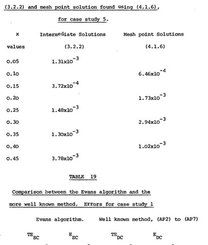
the numerical value of the truncation error for case study 5 where (4.1.6) has been employed.

Truncation Error and Stability conditions for (4.1.6)

The truncation error for the scheme (4.1.6) is obtained in the same manner as for the cases with constant coefficients. It

is, however, much more complex and in fact involves some deriva­ tives of the variable coefficients and also some odd order deriva­

+f-r

2e/ 32a' + 3fb + kf_ / S^a'+B^b \ ^-k20 33c -1 /23c+k^ j^c

3u

+j-r20/

32a + k^_

d**a

\ - k20

32c + h2 3**c + k_^_ 3**c

I U t 2

12 at"/ 12 V 3t2

3x23t2 6 3t"

- f 2c+h2

9fc+h^_

\1 3fu

f -k20 / 32a* + 3fb + kVS^a1

12 V

3x2 12 Sx1*' I 3x2

6 \3t2

3t2

“ Ist"

+ 3 M \ - l(a'+b)- h2k2033c - hf_ / 23c + 3fc \ ) 3ju

3t*'i 6

3

3x3t2 36 V 3x 3 3x3

>

f 3x3

+ J - k20 / 32a+k2 3**a \ - a_ - k2h20 / 232c + h2 S^c + k^ 3*^

\

I H s t 2 12 3tw 12 144 I 3t2

3x2 3t2 6 3t*

- h2

1

2c+h232c + 3*»c

\ \

3**u + f-r20 / 12 3c: + k2 33c

144 V

3x2 12 3x** / J 3x“ \ 6 I 8t

+2h2 33c

\

+ f-k2r20/12 3c +2h2 33c +2k2 33c \] _{33u + ( r2-k2 r20/l2c+8k2 32c} 36 I 3t 3t3x2 3t3 / J 9t3 |12144 I 3t2

+ 2k^

dkc

+k2h2 3**c

3 dtk 3x23t2

\ \

f

\+ k3 /

\

+ j-r20/ 23a+k3 3 3a \ -i-k2 h 0 /2 32c + 1^

| ^ "3t 3 / 6 \ 3t3x 3 (h2+k2) 3_3x3t;4c _3t3xJ3 u

+ J -k2r2 0/2/ 3a1 + 3b \+ k2 / 33a ! + 33b

t2(

3t 3t _{3t; 3tc} 13 8t3x

+ 1 (h2+k2) 3**c

3 _{3x3t /j}\ I 9**u +

_{/ I}

₃

_t

₃₃

_{x )}

₆

₂

_V

₃

_t

₂

₁₂

₃

_{t** /}

- k^ 0/ 2c+2k2 3fc + k^_ 3^c + k2h 2 3 u

3t4 3t 3x23t2 '

J

2 / 1^1 + 9^

3t 3t + k2 / 33a ’ + 33b_{3t; 3t'} - k2 h20 / 2 18 3t3x32c

+ _i (h +k ) 3 c

3 3t3x'

3 u j 3t3x;

(4.2.1)

In addition to this expression from the Taylor series expan­

sion of each term in the scheme (4.1.6), we also have some terms

resulting from the derivation of the scheme itself. These

terms result in the following expression and must be added to

where

B. = -ha'. . + h2 a". . - h 3 a"1. . + h 1* a ,v

3

x'3

T

T ^

C. = -ha". . + h 2 a"‘. . - h 3 a ,v. . - hb’. . + h2 b " . .-h3b'". .

3 j - 1,3 i,3 i,3 2~ g“ 1,3

+ h** b ,v/. .

24 *'3

D. = ha'. . + h 2 a". . + h 3 a"'. . + h*1 a*'' . 3 1,3 y 1,3 g“ 1/3 24 1/3

E. = ha". . + h2 a"1. . + h 3 a'Y . + hb'. .+ h 2 b". .+h3bni 1/3 J~ 1/3 g~ 1,3 1/3 J - _{1,3 6}~ 1,3

+ h4 b tV. . 24 1,3

The von Neumann stability condition for (4.1.6) is obtained

by applying the method locally. This is because the method,

stability condition by considering the coefficients to be con­ stant then it is reasonable to assume that the scheme with

variable coefficients will be stable if the condition obtained is satisfied at every point in the solution domain. Since the

scheme (4.1.6) reduces to (3.2.14) when the variable coeffi­

cients are considered to be constant then the stability conditions

are naturally the same. Thus for the splines scheme (4.1.6) (i) if 0 ^ h it is unconditionally stable

is satisfied independently at each point of the solution domain.

4.3 Comparable Finite Difference Scheme

Again as a comparison to the scheme incorporating splines

we consider the well known finite difference approximation. The

method is analogous to the constant coefficients case described in section 3.5 in that, at (ih,jk), we consider as an approxima­ tion to (4.1.2) the expression

(ii) if 0 < % it is stable when r £{3a(x,t)(1-40)}

(4.2.3)

= 1_ {aa h2

+(l-2a) (a” . ,+b. .)<$ U. ._{1,-3 x 1,3}

j

+ac. . _{i f]-l i,D-l} _u. . - + (l-2a)c. _{i#D 1,3} .u. . + ac. _{1,3+1 1,3+1}u.

(4.3.1)

(i=0,l,„..,N;j=l,2, ... ; N h = l )

where 6 2 U. . = U. . . - 2U. . + U.,. ._{x 1,3 i-l,3 i,3 i+l,3}

and 5 U. . = U . - U. . . ._{x 1,3 1+1,3 1-1,3}

Collecting like terras in (4.3.1) and letting r = k/h we have the tri-diagonal system

J-ar2a. _.+ahr2 /a*. .^,+b. . ..,+/l+2ar2a. ■

< 1,3+1 ~2~ ' 1,3+1 i,3+l > i-l,3+1 i 1,3+1-ak2c. .., lu.’i, j+1) i,j+1

+ j-ar2a. ... - a

(a1.

+ b. ..jlu... ...

\ i,3+l — zr i,3+l i,3+l > i+l,3+1

(l-2a)r2a. (l-2ot)hr2(a'.

.+b.

.)lu.

1 1,3 1,3 1,3 j i-l,3 ^ 1,3

+(l-2a)k2c. .

lu . . +

J

.+b. .)

I

1,3 ? 1,3 | 1,3 -J" 1,3 1,3 j 1+1,3

. . _+ahr2(a'. .

_+b. .

,){u.

l,3-1 ~y ~ 1,3-1 i,3-l f i-l,3-1 | i,3-l i,3-lj

^-ar2ai

U. . . -V-ar2a. . . - ahr2 fa1. . _+b. . .) U.^. . ,_{1,3-1 l i,3-l — i,3-l i,3-l ( i+l,3-1}

4.4 Truncation Error and Stability Conditions for (4.3.2) In the usual manner we expand each term of (4.3.2) about

the mesh point (ih,jk) and thus obtain the expression for the

truncation error

. 2,2

k h -ar%2c+k2 S^c

- ar2/ 32a'+32b+k2

SV+S^b

L \3t2 12 St1* '

\ 3t2 3t2

dt"

St1*

\

J

-ar2r

k2

d^a

3t“ 12

1

(a‘ +b) - k^_ a

6 6 3_3t-a* + 92b_3t‘

+

12 3V_+3^b _{St1* St4} 33u

+ j -

_{'3t2 12}

_dth

- ar2/

a r^_

\ 9t 3 8t3 / 3t 2 3t' 12 3t 3t"

-a k2r2 / 23c+k3 33c \ 3su + f r^_ -a k 2r2 / 2c+k232c+k1* 3^c \ \ 3^u

3t' 3t; 12 24 [ 3t2 12 St1*

-ar

| 3t 3t _{3 . 3t3 3t3 . 3t3x}

+k'

3t2 3t2

+ k2

f

1

-a

2 I"

1

12 j

+ k;

3 33a*+33b '_{3t3 3t3 3t33x} S^u - ar2/23a + k^ 33a_{' 9t 3 3t3 3t3x.'}3 u

- a r;

+ k2 3a + k 3a

34u + . o (4.4.1) 3 i 3t3 9t3 . / 3t3x3

This truncation error (4.4.1)f for the fully implicit finite

difference scheme (4.3.2), is slightly simpler than that for

the scheme incorporating splines. This is due to the fact that there are no terms such as c. _ c. etc. in the finite difference scheme.

The von Neumann stability condition for (4.3.2) is found

by again applying the method locally. Hence by considering the coefficients to be constant we can obtain the following condi­ tions governing stability.

(i) if a > h the scheme is unconditionally stable. (ii) If a < h _{the scheme is stable provided}

is satisfied independently at every point in the solu­

tion domain.

The stability condition (4.4.2) can also be rewritten in the alternative form

This form is used by Saul'yev (1964) when considering parabolic equations with variable coefficients and is equally applicable to the stability condition (4.2.3).

1-1,j i-l,j-l

r < {a(x,t)(l-4a)} 5 (4.4.2)

(4.4.3)

-44-Although our method of obtaining the conditions (4.2.3) and

(4.4.2) is not a rigorous proof of stability it is supported by numerical evidence in the case study 5 where the coefficients are varying throughout the range 0£x£l. A more thorough analysis of stability can be performed using the energy method. It has, in

fact, been shown by Lees (1960) that the finite difference approximation

has the same condition governing unconditional stability as the equivalent scheme for constant coefficients. The stability condi­

tions for (4.4.4) with constant a,b,c,d and e are the same as (3.6.3). Unfortunately the energy method used in the Lees paper

gives no information about the conditional stability of the scheme

although this has since been remedied by Friberg (1961). In his paper, Friberg modified the method used by Lees to examine the conditional stability of (4.4.4) with b(x,t) = c(x,t) = d(x,t)

= e(x,t) = 0. By constructing a system of first order equations equivalent to

+ d(x,t) U. . + e(x,t) _{if D} (4.4.4)

of the equation

3*~u = a(x,t) 32u +b(x,t)3u + c(x,t) 3u + d(x,t)U + e(x,t)

at2 3x2 3t

(4.4.6)

he showed that (4.4.4) (with b=c=d=e=0) is stable for a<h when

which is identical to the condition (3.6.3) governing stability of the scheme for constant coefficients.

These results deribed by Lees and Friberg indicate that the

change from constant coefficients to variable coefficients will not greatly affect the stability conditions for a particular shceme provided that they are satisfied at every point in the

solution domain.

4'. 5 Numerical Procedure and Evaluation of Truncation Errors The numerical procedure for finding cubic spline solutions at points intermediate to mesh points for the equation with

variable coefficients (4.1.1) is almost identical to that given in section 3.7. The only major difference is in deriving the "end conditions", since the continuity expression (3.2.3) will be

unchanged and thus used in the same manner. As an example, the "end condition" (3.7.2) on the boundary x=0 will become

r2 < a(l-4a) (4.4.7)

(4.5.1)

(3.2.1) by (4.1,3) in the general scheme, the remaining procedure

is unchanged.

The estimates of the truncation errors (4.4.1), for the

implicit scheme, and (4.2.1) plus (4.2.2) for the splines echeme are obtained using the method outlined in section 3.8. In this case, however we have to evaluate the derivatives of the variable coefficients with respect to both x and t and also some mixed derivatives of the coefficient c(x,t). This is easily done using difference approximations similar to (3.8.1) provided the variables

a(x,t),b(x,t) and c(x,t) are sufficiently differentiable. Assuming this is so, then it can be seen that the truncation errors (4.2.1) and (4.4.1) are both © ( k ^ 2) as was the case for the equivalent

schemes with constant coefficients. The expression (4.2.2) which is added to (4.2.1) to give the full truncation error for the

2

scheme (4.1.6), is 0(k h) although in practice it should be noted that the numerical values of these truncation errors will greatly

depend on the actual values of a, b and c.

When obtaining an estimate of the truncation error for the

splines scheme (4,1.6) we must first use the numerical procedure to find values for the M's and L's since these are required in (4.2.2)

^•6 Singularities in the variable coefficients

It is sometimes the case that one or more of the variable coefficients a(x,t), b(x,t) or c(x,t) will have a singularity at a point in the range 0 < x £ 1. This problem is best discussed using an example due to Collatz (I960), where the equation under consideration is given by (4.1.1) with a(x,t) = 1, b(x,t) = 1/x

and c(x,t) =0. In this case finite difference approximations

require special consideration at the singular point x = 0. One

method is to employ L' Hospital's rule, which in this case gives

lim 3u/3x = lim 32u/3x2

x^° x xr>° 1

x=o

(4.6.1)

whereby the differential equation becomes at x=0

2 32u = 32u (4.6.2)

3x2 3t2

A finite difference scheme can now be used to approximate (4.6.2) and hence the problem has been removed. In a similar manner other singularities occuring in (4.1.1) can be dealt with and the schemes (4.1.6) and (4.3.2) modified to give the required solutions. The

equation under consideration in case study 5 does in fact have a

singularity at x=2 since the coefficient b(x,t) = 2(x-2) \

Fortunately this poses no problem in this instance since the equa­ tion (4.1.1) has only been considered in the range 0 ^ x ^ 1.

CHAPTER 5

Unequal Step Lengths

5.1 General Considerations

As indicated in section 2.2 the knots x^ (i « 0,1,...,N) need

not necessarily be equally spaced in the range a £ x £ b. The

distance between successive knots given by

h^ = x^ - xj»i ^ s 1#2/...,N) (5.1.1)

is chosen as the constant value h in chapters 3 and 4 simply because

it is usual in deriving finite difference approximations to have a constant step length. As will be shown in this chapter both the well known finite difference scheme and the scheme incorporating splines can be generalised to the case of non-uniform step lengths.

Before deriving these latter schemes it is convenient to first consider the relative merits of employing a variable mesh; the main

Here, as suggested by Saul'yev (1964), we would use a smaller step length h in the first third of the interval [o,l] them in the

remaining two thirds. This is because the function is varying

rapidly in the first third of the interval and hence more solution values are required. The alternative to using variable step lengths

in this case, is to employ a very small constant step length through­ out the range £o,lj and thus obtain the required solutions. This is very uneconomical with regard to computing time since the number

of arithmetical operations is greatly increased and thus a variable step length scheme is desirable.

The major disadvantage of using a non-uniform mesh to solve partial differential equation is that the schemes produced are rather more complex and are also likely to have a larger error.

The reason for this is that there are errors associated with all finite difference approximations which usually depend on the size of

the step length h. If we therefore increase h in one portion of the range so as to decrease it in another than the order of the error will still depend on the larger step length used. This is

also the case in the finite difference schemes incorporating splines since the spline function is, by definition, a piecewise polynomial

in each of the intervals between successive knots. If we therefore increase the distance between knots in one part of the range then we would naturally expect the truncation error to be large in that vicinity. We have found that this can be counteracted to some

extent in our schemes by choosing the parameters a and 6 to eliminate

some terms in the truncation errors. This technique is discussed

An additional advantage of employing schemes with unequal mesh lengths may occur when the equation (4.1.1) has a singularity in one of the variable coefficients. As indicated by Ames (1969), a very common method of dealing with this type of problem is to

attempt to diminish the effect of the singularity by refining the

mesh in the region where it occurs. Thus by reducing the size of

the step length around the singularity we minimize the hrea of

infection' it causes. If we were solving a problem of this type using either of the constant step length schemes (4.1.6) or (4.3.2) we would have to reduce the size of the mesh throughout the whole

range 0 £ x C 1. This is again very uneconomical with regards to

computing time, particularly when a large amount of solutions are not required in the x direction. It would therefore be useful if

we had a scheme with variable step lengths where we could use small mesh widths around the singularity and larger mesh widths in the remainder of the range.

5.2 Cubic Spline Finite Difference Approximation to (3.1.1)

Recalling the results of Ahlberg, Nilson and Walsh (1967),