Munich Personal RePEc Archive
The Use of Pseudo Panel Data for
Forecasting Car Ownership
Huang, Biao
Department of Economics, Birkbeck College, University of London
June 2007
The Use of Pseudo Panel
Data for Forecasting Car
Ownership
Biao Huang
Birkbeck College, University of London
Thesis Submitted in Accordance with the Requirements for
The Degree of Doctor of Philosophy
Declaration
Acknowledgement
I would like express my extreme gratitude to my supervisor, Prof. Ron Smith, whose insight and constructive comments have proved invaluable. Without his guidance and supervision, the completion of this thesis would be impossible.
The early research findings were presented to the European Transport Conference in 2005. The comments from various seminar participants as well as Dr. Walter Becket of Birkbeck College are gratefully received.
I also thank Dr. Gerard Whelan for generously supplying a copy of his PhD thesis. This work also benefits indirectly from my other projects work with colleagues at the Transport Studies Unit, University of Oxford, MVA Consultancy and Mr. John Bates. I thank them for their unknowing contributions.
Abstract
While car ownership forecasting has always been a lively area of research, traditionally it was dominated by static models. To utilize the rich and readily available repeated cross sectional data sources and avoid the need for scarce and expensive panel data, this study adopts pseudo panel methods. A pseudo panel dataset is constructed using the Family Expenditure Survey between 1982 and 2000 and a range of econometric models are estimated. The methodological issues associated with the properties of various pseudo panel estimators are also discussed.
For linear pseudo panel models, the methodological issues include: the relationship between the pseudo panel estimator and instrumental variable estimator based on individual survey data; the problem of measurement errors (and when they can be ignored) and the consistent estimation of dynamic pseudo panel parameters under different asymptotics. Static and dynamic models of car ownership are estimated and a systematic specification search is carried out to determine the model with best fit. The robustness of the estimator is investigated using parametric bootstrap techniques.
As an individual household’s car ownership choice is discrete, limiting the model to linear form is obvious insufficient. This study attempts to combine the pseudo panel approach with discrete choice model, which has the distinctive advantages of allowing both dynamics and saturation but without the need for expensive genuine panel data. This does not seem to have been done before. Under the framework of random utility model (RUM), it is shown that the utility function of the pseudo panel model is a direct transformation from that of cross-sectional model and both share similar probability model albeit with different scale. This study also explores the various forms of true state dependence in the dynamic models and tackles the difficult econometric issues caused by the inclusion of lagged dependent variables. The pseudo panel random utility model is then applied to car ownership modeling, which is subsequently extended to take saturation into account. The model with the best fit has a Dogit structure, which is consistent with the RUM theory and is able to estimate the level of saturation and test its statistical significance.
Table of Content
Chapter 1 Introduction ... 10
Chapter 2 Review of Car Ownership Models... 15
2.1 Static Model ... 16
2.1.1 Aggregate trend extrapolation model (GB: pre 1970s)... 16
2.1.2 Partially disaggregate model (GB: 1970s and 80s)... 18
2.1.3 Fully disaggregate models (GB: 1990s and beyond) ... 18
2.1.4 Models of Car Ownership and Types ... 20
2.1.5 Models of Car Ownership and Types allowing for Heterogeneity ... 21
2.1.6 Joint Estimation of Car Ownership and Use ... 22
2.2 Dynamic Models ... 23
2.2.1 Time series Models ... 24
2.2.2 Equilibrium Market Models... 24
2.2.3 Panel Data Model (of car holdings) ... 25
2.2.4 Pseudo Panel Models ... 27
2.2.5 Dynamic Transactions Models... 29
2.3 Conclusion ... 32
Chapter 3 Pseudo Panel Data... 33
3.1 Family Expenditure Survey... 33
3.2 Factors Influencing Car Ownership ... 35
3.3 Constructing the Pseudo Panel Dataset... 36
3.4 Examining Pseudo Panel Variables ... 38
3.4.1 Number of Cars Owned or Used by the Household... 39
3.4.2 Average Weekly Public Transport Expenditure per Person ... 41
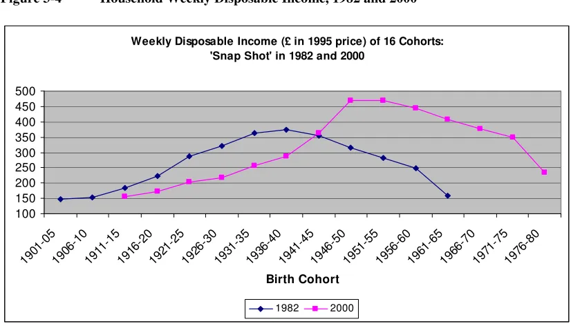
3.4.3 Weekly Household Disposable Income ... 42
3.5 Aggregate Time Series Data ... 43
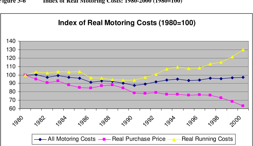
3.5.1 Motoring Costs... 43
3.5.2 Demographic Data ... 44
3.6 Conclusion ... 45
Chapter 4 Measurement Error and Linear Static Fixed Effect Model... 46
4.1 Weighted Least Square Estimator... 46
4.2 Consistent Estimation of FEM with Measurement Error... 49
4.3 Conditions to Ignore Measurement Error Problem... 51
4.4 Empirical Results from Static Car Ownership Model... 54
4.4.1 Models based on Weighted Least Square Estimator... 56
4.4.2 Models Based on Genuine Panel Data Estimators... 61
4.5 Conclusion ... 68
Chapter 5 Linear Dynamic Model ... 70
5.1 Consistent estimator of dynamic pseudo panel model... 70
5.1.1 Cohort Dummy IV estimator ... 71
5.1.1.1 Error Corrected Within-Group Estimator ... 73
5.1.1.2 Error Corrected GMM Estimator ... 74
5.1.1.3 Within Group Estimator... 75
5.1.2 Estimator based on individual level data ... 78
5.1.2.1 Two-Stage Least Square Estimator by Moffitt ... 78
5.1.2.2 GMM Estimator of Quasi-differences Model ... 79
5.2 Empirical Results from the Dynamic Car Ownership Model ... 80
5.2.1 Assuming linear economic relationship at individual level ... 81
5.2.2.1 Specification Search... 85
5.2.2.2 Results of the Preferred Models... 88
5.2.2.3 Alternative Model Specification and Estimation ... 91
5.3 Conclusion ... 94
Chapter 6 Random Utility Model of Pseudo Panel... 97
6.1 Pros and Cons of Nonlinear Pseudo Panel Models... 97
6.1.1 Nonlinear and Linear Pseudo Panel Models ... 98
6.1.2 Pseudo Panel and Cross Sectional Models... 99
6.2 A Random Utility Model of Car Ownership... 102
6.2.1 Random Utility Model of Pseudo Panel... 103
6.2.2 A Discrete Choice Model of Household Car Ownership... 107
6.3 Estimation of Discrete Choice Pseudo Panel Model ... 111
6.3.1 Fixed Effect model... 112
6.3.2 Random Effect Estimators ... 115
6.4 Empirical Results of Static Car Ownership Model ... 117
6.4.1 Models of One Plus Cars ... 118
6.4.2 Models of Two plus Cars Conditional on Owning the First Car ... 126
6.5 Conclusion ... 131
Chapter 7 Dynamic Model and Model with Saturation... 133
7.1 Dynamic Random Utility Model of Pseudo Panel... 134
7.1.1 Standard State Dependence Model ... 136
7.1.2 Models of Propensity Dependence ... 136
7.1.3 Models of Dynamic Optimisation... 138
7.1.4 Transforming the Reduced Model for Repeated Cross Sections ... 139
7.2 Consistent Estimation of Dynamic Model ... 142
7.2.1 Literature Review on Genuine Panel Model... 143
7.2.1.1 Fixed Effect Models and Incidental Parameter Problem ... 143
7.2.1.2 Random Effect Model and Initial Condition Problem ... 145
7.2.1.3 Semi-Parametric Model ... 147
7.2.2 Estimation Methods Proposed for the Current Study ... 148
7.3 Empirical Results of Dynamic Car Ownership Model ... 153
7.3.1 Dynamic Model of One plus Car ... 153
7.3.2 Dynamic Model of Two plus Cars ... 161
7.4 Model with Saturation ... 163
7.4.1 Dogit Model ... 164
7.4.2 Empirical Results of Car Ownership Model with Saturation... 166
7.5 Conclusion ... 170
Chapter 8 Car Ownership Forecasts ... 173
8.1 Projection of Explanatory Variables ... 174
8.1.1 Forecast Assumptions ... 174
8.1.2 Generating Projections of Input Variables... 175
8.1.3 Checking of Projection Results... 177
8.2 Car Ownership Forecasts and Model Performance Evaluation .... 178
8.2.1 Selection of Econometric Models ... 179
8.2.2 Forecasting and Validation ... 181
8.2.3 Forecasts Evaluation and Sensitivity Test... 185
8.3 Conclusion ... 191
Reference... 198
Appendix 1 Supplementary Tables and Figures ... 210
Appendix 2 Gauss Code for Pseudo Panel Mixed Logit Model... 217
List of Figures
Figure 3-1 Average Number of Cars for two Cross Sections of Cohorts: 1982 and 2000 ...40
Figure 3-2 Average Number of Cars per Household, Profile by Age of Household Head from Eight Cohorts...41
Figure 3-3 Average Weekly Public Transport Expenditure per Person, 1982 and 2000...41
Figure 3-4 Household Weekly Disposable Income, 1982 and 2000 ...42
Figure 3-5 Weekly Disposable Income: Age Profile from Eight Cohorts...43
Figure 3-6 Index of Real Motoring Costs: 1980-2000 (1980=100) ...44
Figure 3-7 Total Number of Households and Average Household Size: GB 1980-2000 ...45
Figure 4-1 Regression Residual Plot of the Fixed Effect Model...59
Figure 4-2 Fixed effects in the linear model ...62
Figure 4-3 Residual Plot of unrestricted Fixed Effect Model ...65
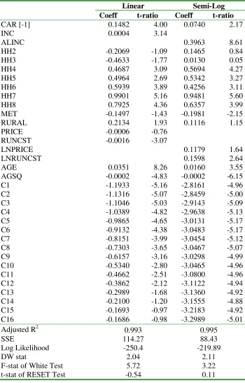
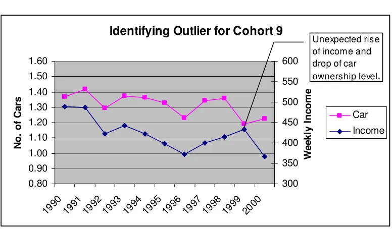
Figure 5-1 Residual Plot of Semi-Log Model with outlier...87
Figure 5-2 Identifying outlier for cohort 9 in year 1999 ...87
Figure 5-3 Residual Plot of the unrestricted fixed effect model...90
Figure 5-4 Log Income Variable: distribution of the simulated coefficients and point estimate based on real data ...93
Figure 5-5 Log Running Costs Variable: distribution of the simulated coefficients and point estimate based on real data ...93
Figure 5-6 “Most Likely” fixed effects from simulation and point estimate from real data ...94
Figure 6-1 Two Structures of multiple car ownership modelling ...109
Figure 6-2 Observed and Predicted probability of household owning 1+ car by income ...123
Figure 6-3 Residual against household income...124
Figure 6-4 Residual against Household Income (Model 3, Car 2+|1+)...129
Figure 7-1 Marginal Effects of Cohort Dummies (Model 14) ...157
Figure 7-2 Residual plot of the Random Parameter model ...159
Figure 7-3 Residual Plot of the Car 2+|1+ Model ...162
Figure 7-4 Choice Set when some decision makers are constrained not to own a car ...165
Figure 8-1 Projected weekly disposable income: Profile by age of household head ...178
Figure 8-2 Projected average household size: profile by age of household head...178
Figure 8-3 Observed Total Car Stocks and Forecasts from four Models ...184
Figure 8-4 Model L1: Average Number of Cars per Household, X-axis by cohort age ...186
Figure 8-5 Model D1: Proportion of Households Owning 1+ Car, X-axis by cohort age...188
Figure 8-6 Model D3: Proportion of Households Owning 2+|1+ cars, X-axis by cohort age ...188
List of Tables
Table 1-1 Common Notations ...13
Table 3-1 Data Coverage Summary of FES ...34
Table 3-2 Definition of eight household types ...36
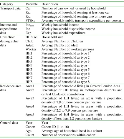
Table 3-3 Variables in the Pseudo Panel Dataset ...39
Table 4-1 Descriptive statistics of the variables...56
Table 4-2 Regression results of Pooled WLS model and Fixed Effect Model ...58
Table 4-3 Linear Model: Unrestricted and restricted Fixed Effect Model...63
Table 4-4 Income and Price Elasticity (based on Semi log, unrestricted FE model)...65
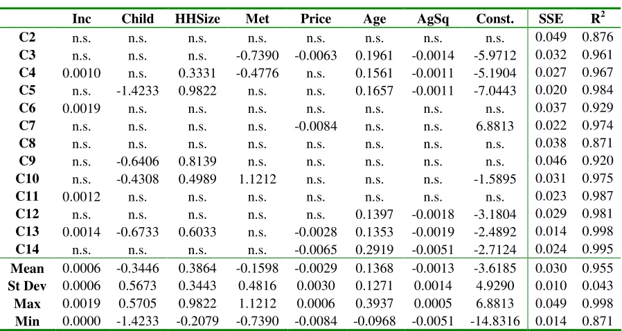
Table 4-5 Cohort Specific Regression Results (Linear form; 13 cohorts) ...67
Table 5-1 Models with best fit (comparison of linear and semi-log functional form)...83
Table 5-2 Short Run and Long Run Income Elasticity...86
Table 5-3 Short Run and Long Run Running Cost Elasticity...86
Table 5-4 Unrestricted and restricted fixed effect model (semi log form) ...89
Table 5-5 Model Specification and LDV Coefficient ...89
Table 5-6 Comparison of elasticities (dynamic and static unrestricted FE models)...91
Table 6-1 Advantage and Disadvantage of nonlinear pseudo panel model ...102
Table 6-2 Logit Model 1-4, alternative variables for household characteristics and location (t-stat in the parenthesis)...119
Table 6-3 Marginal Effect at weighted average of explanatory variables, Model 1 – 4...121
Table 6-4 Income, price and running costs elasticity for household with various income...121
Table 6-5 Models with Log Income and Log price variables (t-stat in parenthesis) ...124
Table 6-6 Elasticity derived from models with log income and log price variable ...125
Table 6-7 Descriptive Statistics of Pseudo Panel Dataset 2 ...127
Table 6-8 Results of Model with Detailed Location Variables and Linear Income variable (t-stat in the parenthesis)...128
Table 6-9 Income and Price Elasticity (Model 2 & 3 with linear income and price variable) ...128
Table 6-10 Model 2+|1+ with Log Income and Log Price Variables (t-stat in the parenthesis) ...130
Table 7-1 Summary of Initial specification search ...154
Table 7-2 Fixed Effect Models with Log Income and Cost Variables (t-stat in parenthesis) ...156
Table 7-3 Short run elasticity derived from FE models with log income and price variables ...156
Table 7-4 Long run elasticity derived from FE models with log income and price variables...158
Table 7-5 Results of Random Parameter Model (t-stat in parenthesis) ...158
Table 7-6 Short Run and Long Run elasticity based on the mean of random parameters ...160
Table 7-7 Random Parameter Model for Car 2+|1+ (t-Stat in parenthesis) ...162
Table 7-8 Income and cost elasticity for model of Car 2+|1+ ...163
Table 7-9 Forecasting model of one plus cars (t-statistic in parentheses) ...168
Table 7-10 Short run and long run income elasticity of one plus car model...168
Table 7-11 Model of Car 2+|1+ (t-stat in parenthesis) ...169
Table 7-12 Income and cost elasticity of Car 2+|1+ ...170
Table 8-1 Parameters of Econometric Models Used in Forecasts...181
Table 8-2 Multiple-car factor used in forecasting ...182
Table 8-3 Observed Total car stock vs. forecasting results (000s) ...183
Table 8-4 Proportion of Households with zero, one and two plus cars ...185
Table 8-5 Forecasts Comparison: current studies vs. published studies (millions) ...185
Table 8-6 Sensitivity Test: GDP growth is 0.5% higher per annum...190
Chapter 1
Introduction
The car market is an important sector of most modern economies and both the demand for ownership and the demand for new cars play an important role in economic decisions. The health of the car industry in general depends on consumers’ demand for new cars. Demand forecasting is one of the most important tools car manufacturers use in their financial planning and decision making about expansions and contractions of plant capacity. For various government and public bodies, understanding and forecasting demand for car ownership are equally important. As the most important user of petroleum fuel, the car market has a strong influence on non-replaceable energy. Projections of future fuel consumption, and the impacts on fuel consumption of various forms of government intervention, are routinely based on forecasts for car ownership demand. Furthermore, understanding the factors driving demand for cars is important in addressing a range of environmental issues including local air pollution and climate change. Since car emissions are a large component of pollution, air quality standards and policies are largely based upon projected car ownership and use. Finally, accurate car demand models are also an aid to planners who must anticipate infrastructure needs, address concern of congestion and provide public transport services. Government agencies and local passenger transport authorities utilize projections of car ownership levels as a key input to obtain accurate projections of infrastructure needs and public transport patronage.
highly significant in mature markets. It is easier to understand these points by looking at the car market in Great Britain as an example. Between 1950 and 2005, the total number of cars in the stock increased from 1.98 million to 26.21 million, implying an average growth rate of 4.7% per annum; for the same period, the real Gross National Income (GNI) increased from £243 billion to £987 billion (1995 prices), implying an average growth rate of 2.5% per annum (DfT, 2006c; ONS, 2007). If one uses certain time series models (for example, a simple Error Correction Model) for long term forecasts, it would substantially over-estimate the car stock in distant future. This is because the past growth trend will be inevitably curtailed by the approach of saturation: in 1951, only 14% of households had regular access to at least one car, while this proportion increased to 75% in 2004 (DfT, 2006c).
In the current study, the car demand forecasting model is developed within the context of British car market. In the UK, the Department for Transport has commissioned a number of “official” forecasting models over the past few decades, which include those developed by the Transport and Road Research Laboratory, the Regional Highway Traffic Model (RHTM), the National Road Traffic Forecasts (NRTF) and the National Transport Model (NTM). Besides the Department for Transport, there are industrial organisation such as SMMT (The Society of Motor Manufacturers and Traders) and other commercial and academic organisations, which are also involved in this area of research. However, some of the research remains “in house”, i.e., the details of the model are not publicly available. Some of the studies available in the academic journals used methodology and data different to the NRTF/NTM, yet each study has its own limitations. Various types of car demand forecasting models developed in Great Britain and worldwide will be reviewed in Chapter 2.
of habit, imperfect information regarding alternatives and prices, costs of adjustment and transaction costs, have been empirically assessed.
Nevertheless, the use of dynamic approach in car demand forecasting is still limited due to heavy data requirements. Due to data constraint, there have been relatively few forecasting models that use the dynamic approach except those using aggregate time series methods. It is possible to forecast car demand using panel data models. However, there is only one panel survey in Britain containing limited transport related information: the British Household Panel Survey (BHPS), which is inadequate for the purpose of our study. Furthermore, due to the attrition problem, the size and representativeness of the samples decline over time, rendering the panel data inferior to other national cross-sectional data. For example, less than half of the respondents in Wave 1 of BHPS remained in the sample in Wave 13, and various population groups such as the old, the young, the unemployed, those with low income, etc. became significantly under-represented (ISER, 2006).
One approach to circumvent the need for panel data is to construct pseudo panels from the cross sectional data. The pseudo-panel approach is a relatively new econometric approach to estimate dynamic demand models. A pseudo-panel is an artificial panel based on (cohort) averages of repeated cross-sections. The cohorts are defined based on time-invariant characteristics of the households and extra restrictions should be imposed on pseudo-panel data before one can treat it as genuine panel data. Using the cohort data over a number of periods, one could distinguish long run and short run effects while allowing for heterogeneity between the cohorts. In this way, one is able to overcome the deficiencies in both the static models and aggregate time series.
the pseudo panel cohort data? In many cases, e.g. logarithmic transformations, the average of the transformed data is not defined, since the micro data contain zeros1. Is it possible to apply the microeconomic theory of utility maximization for individual decision makers and combine the pseudo panel model with the random utility model? What are the pros and cons of discrete choice (nonlinear) pseudo panel model and what’s its relationship to standard random utility models? How can the nonlinear pseudo panel model be consistently estimated? And finally, what are the empirical appeals of the pseudo panel models and how well do they perform in car ownership forecasting?
To facilitate readers’ understanding, we list the most common notations that are used throughout the thesis in Table 1-1. The following subscripts are consistently used: i
denotes the individual household in the micro survey; c denotes the associated cohort of household i; and t denotes years.
Table 1-1 Common Notations
Notation Description
Act Average number of cars (automobiles) per household in cohort c in year t P1+ Probability of household owning at least one car
P2+|1+ Probability of household owning two or more cars conditional on owning
at least one car
nct Number of sample observations in cohort c in year t
Nc Total population of cohort c (assumed to be constant in the theoretical
model, i.e. no birth or death)
C Total number of cohorts
Scalar: coefficient for the lagged dependent variable
✁
K x 1 vector of coefficients for exogenous explanatory variables
✂
Unobserved cohort heterogeneity (fixed effect or random effect)
In the empirical work, the dependent variable is Act for all linear models. It is slightly
more complicated for discrete choice models. We observed the proportion (not
probability) of households owning at least one car in cohort c in year t, which is noted as 1+
ct
r . Among the car owning households in cohort c, we also observed the proportion
of those owning two or more cars, which is noted as 2+|1+ ct
r . They are the dependent
1
variables in two separate discrete choice pseudo panel models. The first order condition of the maximum likelihood function implies that the predicted probability (P1+ and
P2+|1+) equals the proportions (rct1+ and
+ +|1 2 ct
r ) in the sample under certain conditions (e.g. probability model is a multinomial logit model with alternative specific constant).
The thesis is organized as follows. Chapter 2 is the literature review of car ownership models. Chapter 3 describes the data used in the thesis including the construction of the pseudo panel dataset. Chapter 4 discusses the linear static fixed effect models, investigating the relationship between the pseudo panel estimator and the instrumental variable estimator based on individual survey data as well as the measurement error problems (and when they can be ignored). Chapter 5 discusses the consistent estimation of linear dynamic pseudo panel model under different asymptotics and the rank conditions for identification. For empirical models of car ownership, systematic specification search is carried out to investigate various issues such as appropriate explanatory variables, functional forms, problems of heteroskedasticity and autocorrelation, fixed or random effects and presence of heterogeneity.
Chapter 6 extends the pseudo panel approach to discrete choice model. The pros and cons of nonlinear pseudo panel model are discussed and a pseudo panel model that is consistent with random utility theory is presented. Chapter 7 investigates dynamic discrete choice model of pseudo panel. Models with different forms of (true) state dependence are compared and consistent estimation methods are proposed for the preferred first order Markov model. For the car ownership model, saturation is an important concept so the theoretical model has been extended and a pseudo panel Dogit model is presented. Empirical models of households with at least one car and those with two or more cars conditional on owning the first car are estimated separately.
Chapter 2
Review of Car Ownership Models
In the chapter, the car ownership models are reviewed. In an early literature review by Train (1986), the methodology found in the literature was divided into two categories: disaggregate and aggregate. The disaggregate method comprises of compensatory and non-compensatory model. In the compensatory models, the household is assumed to trade off characteristics in the sense that a high value of one characteristic can compensate for a low value of another characteristic (for example, the household would choose a car that is smaller than it wants if the price is sufficiently low). The compensatory models can be based on either real choice situations (Revealed Preference Studies) or hypothetical choice situations (Stated Preference Studies). In the non-compensatory models, the consumer is assumed to have an importance ranking of characteristics of the alternatives, and, for each characteristic, have some minimum acceptable level, called a “threshold”. In the decision making process, the consumer eliminates from consideration all the alternatives that do not meet the minimum acceptable standard (threshold) for the characteristic which he considers most important. If more than one alternative remains after the initial elimination, then the consumer looks at his second ranked characteristic and eliminates any alternatives that are not above the threshold for this characteristic. This process continues until only one alternative remains; this is the alternative which the consumer chooses.
Rand (2002) and De Jong et al (2004) classified the car ownership model into nine different types: Aggregate time series model, cohort model, aggregate market model, heuristic simulation model, indirect utility model, static disaggregate choice model, panel model, pseudo panel model and dynamic transaction model. These different model types are then compared based on a number of criteria: inclusion of demand and supply side of the car market, level of aggregation, dynamic or static model, long- or short-run forecasts, theoretical background, inclusion of car use, data requirements, treatment of business cars, car-type segmentation, inclusion of income, of fixed and/or variable car costs, of car quality aspects, of licence holding, of socio-demographic variables and of attitudinal variables, and treatment of scrappage.
Train (1986) and Rand (2002) are both comprehensive surveys of car ownership models, while the literature review here is more focused. More specifically, we cover forecasting models in Great Britain, joint models of ownership and vehicle type/use and different classes of dynamic models. The literature review is organized in two broad categories: static models and dynamic models.
2.1
Static Model
In this section, we first review the “official” car ownership forecasting models in Great Britain, then move on to various advanced discrete choice models. The official forecasting models follow an evolution path of aggregate, partially-disaggregate to disaggregate models2. Beyond the simple disaggregate models (typically Multinomial Logit Models), advanced discrete choice models include joint models of car ownership and types (typically Nested Logit Models); models of car ownership and types allowing for heterogeneity (typically Mixed Logit models) and joint estimation of vehicle ownership, types and use (continuous/discrete model).
2.1.1 Aggregate trend extrapolation model (GB: pre 1970s)
In Britain, the very early car ownership forecasts were on the whole unconditional, i.e. they were single-valued estimate without considering the influences of economic and
2
policy variables (Tanner, 1978). The first formal car ownership forecasting model for Britain is Tanner (1958), which is an aggregate model of trend extrapolation3.
When applying the extrapolation techniques, it has been recognized that car ownership rates should not increase indefinitely in time due to saturation effects. For this reason, Tanner (1958) pioneered a logistic model that relates car ownership rate (cars per capita Ct) with a time trend t:
) exp( 1 0 0 0
0 S t
C S g C C S S Ct ⋅ ⋅ − − ⋅ − + = (1)
Where C0 is the average number of cars per capita in the base year;
g0 is the marginal growth of average number of cars per capita in the base year
(calculated by
dt dC C
1
evaluated at t0);
S is the saturation level.
As a result, knowing C0 and g0 in the based year would enable one to extrapolate Ct in
future years provided the saturation level S can be estimated (although the estimation of S turned out to be problematic and unreliable).
In response to the criticism of Model (1) being too simplistic, Tanner (1978) extended the trend extrapolation model to include the impact of income and motoring costs:
)] ( exp[ ) ( ) ( 1 0 0 0 0 0 t t S a P P I I C C S S C cS bS t − ⋅ ⋅ − ⋅ ⋅ ⋅ − + = − − (2)
where I is the real GDP per capita, P is the real motoring costs and I0 and P0 are the
corresponding values in the based year. So, besides the saturation level S, parameters a,
b, and c should also be estimated.
3
2.1.2 Partially disaggregate model (GB: 1970s and 80s)
In the 1970s, the shortcomings of the aggregate trend extrapolation models were increasingly recognised. The response was to introduce a “partially disaggregate” cross-sectional models while handling the time trend separately using time series approach. Two prime examples are Regional Highway Traffic Model (RHTM, described in Bates, et al. 1978 and cited in Ortuzar and Willumsen, 2001) and 1989 National Road Traffic Forecasts (NRTF).
In RHTM, car ownership was defined as a function of real income deflated by a real car price index, and separate models have been estimated for percentage of households with one plus car (P1+) and percentage of households with two plus cars (P2+):
] ) ( exp[ 1 ) 1 ( ) 1 ( 1 1 b t t t P I a S P − ⋅ − + + = + (3) ) exp( 1 ) 2 ( ) 2 ( 2 2 t t t P I b a S P ⋅ − − + + = + (4)
The model was calibrated on the basis of national, regional and zonal averages data in Britain for the period of 1979-1975 and hence was a “partially disaggregate” model. The model was found to be stable over time, although the same difficult task of estimating the saturation level remains.
The NRTF (1989) maintained the structure of RHTM. It was supplemented by a “separate identification of time trend” (SIC) model, which use the 1985-1986 National Travel Survey data to establish the effect of income hence isolating the time trend effect.
2.1.3 Fully disaggregate models (GB: 1990s and beyond)
• National Road Traffic Forecasts, 1997
NRTF (1997) considered five possible methods in car demand forecasting, which include aggregate time series models, joint models of car ownership and use, panel surveys, group cross-section models and individual cross-section models. The method chosen is the individual (household) cross-section model, in which the probability of car ownership at different household income levels is modelled by a logistic function.
In NTRF (1997), two binary models were calibrated for each household type: a P1+
model to predict the probability of the household owning at least one car, and a P2+|1+
model, defining the conditional probability of the household owning two or more cars, given that they own at least one car:
) exp(
1 1
1 1
LP S P
− + =
+ (5)
) exp(
1 2
2 1
| 2
LP S P
− + =
+
+ (6)
The ownership models included saturation levels of maximum car ownership (S1 and S2
for 1+ car and 2+|1+ cars respectively), and linear predictors (LP) which comprised a linear combination of explanatory variables. The model variables were licences per adult, household income and area type.
• National Transport Model (Previously known as NRTF 2001)
Car ownership forecasting in the National Transport Model was described in Whelan (2001, 2003 and 2007) and included various incremental improvements of NRTF (1997). It accounted for the increase in multi-vehicle households by introducing an additional sub-model, which model the conditional probability of a household owning three or more vehicles (P3+|2+|1+). Unlike the 1997 NRTF, multiple car ownership by
Saturation levels have an important impact upon the results of ownership models. The 1997 NTRF models had allowed variation by household type, but not area type. In the National Transport Model, saturation levels varied according to both household type and area type. Saturation levels were estimated from Family Expenditure Survey data (see Whelan et al. 2000). A general pattern of higher saturation levels in more sparsely populated areas was observed for each model type. Furthermore, a distinct “London” Effect was found, i.e. saturation levels in the Greater London area were lower than in other area types.
2.1.4 Models of Car Ownership and Types
While NRTF (1997) and NTM are fully disaggregate models, they are relatively simple modelling systems, which consist of two or three separate binary choice models (model of Car 1+, Car 2+|1+ and Car 3+|2+|1+). Beyond the simple Binary Logit and Multinomial Logit Models, a number of studies used more advanced discrete choice models to account for correlation between alternatives. In particular, if the household car types are considered in the model, the assumption of independently identically distributed error term in the multinomial logit models is likely to be violated. In this case, the Nested Logit Model, which allows more flexible error structures, becomes a natural candidate. A Nested Logit Model is appropriate when the set of alternatives faced by a decision maker can be partitioned into subsets, called nests, in such a way that: 1) The Independence from Irrelevant Alternative (IIA) property holds within each nest; 2) IIA does not hold in general for alternative in different nests (Train, 2003).
Train (1986) is a modelling system that allows simultaneous estimation of vehicle numbers and types (the model also estimates car use defined as vehicle miles traveled). It has a Nested Logit Structure, where the choice set in the upper nest includes 0, 1 and 2 cars. In the lower nest, the choice set for one vehicle households includes class/vintage of vehicle, while the choice set for two vehicle households includes class/vintage of pairs of vehicles. The household chooses the number of vehicles to own and the class/vintage of each vehicle so that the conditional indirect utility function is maximized.
with the vehicle choice decision decomposed into three linked choices: type-mix, body-mix and fleet size (0, 1, 2, 3 or more vehicles). The utility from holding a car bundle can be represented by a conditional indirect utility function, which includes the following variables: consumption prices, qualities, household wealth, expected annualized vehicle capital costs and socio-demographic factors. A particular bundle will be chosen if the utility flows from it exceed the utility obtained from any other car bundles. A car bundle is decomposed into holding of different fleet size, different body types and different models/vintages. The error terms are allowed to be correlated across bundles with different fleet size, body and model/vintage mixed, but are assumed to be IID for bundles with the same choice mixes.
2.1.5 Models of Car Ownership and Types allowing for Heterogeneity
The impacts of household heterogeneity and random taste variations on household car holdings are attracting more and more attention in recent literature. Because of the rapid development in computing technology in recent years, heterogeneous models can now be estimated using simulation without too much difficulty. Among them, Mixed Logit is a highly flexible model that can approximate any random utility model (McFadden and Train, 2000). It allows for random taste variation, unrestricted substitution patterns, and correlation in unobserved factors over time, which alleviated the three limitation of standard logit. This flexibility gives mixed logit model great advantage in terms of modeling vehicle number and types while allowing for random taste variations. It can also be a highly efficient model in combining revealed preference (RP) and stated preference (SP) data.
In Brownstone et al. (2000), multinomial logit (MNL) and mixed logit models were compared based on data on Californian households’ revealed and stated preferences for cars. In the vehicle choice modeling context, they found RP data was critical for obtaining realistic body-type choices and scaling information. SP data was critical for obtaining information about attributes not available in the marketplace, but pure SP models gave implausible forecasts.
multiplier test from McFadden and Train (1997) was used. Five random coefficients were identified, amongst which four were applied to the different vehicle fuel types modeled, demonstrating large heterogeneity in taste for alternative fuel vehicles. The RP models were also estimated separately. The model result showed that only terms for price and operating cost could be determined with any accuracy due to high co-linearity between vehicle range, speed and acceleration. Joint SP/RP models were then estimated. A scale factor was used to scale the SP data relative to the RP data. While this scale factor is less than one for the MNL model, it is greater than one for the mixed logit model, where the preference heterogeneity is captured by fuel-type error components.
The authors proceeded to make new vehicle forecast for California. The mixed logit models tend to result in higher market shares for the alternative fuel vehicles. A key point here is that the IIA properties of the MNL means a proportionate share of each new vehicle’s market share must come from all other vehicles, whereas the mixed logit specification results in the more plausible result that the market share for electric fuel vehicles comes disproportionately from other mini and subcompact vehicles.
2.1.6 Joint Estimation of Car Ownership and Use
While household’s car ownership decision is discrete, vehicle use is continuous. A special type of random utility model, joint continuous/discrete model, was developed for this situation (Dubin and McFadden, 1984; Train, 1986). Household’s decision on car ownership and use is jointly depicted by a “conditional indirect utility function” and a demand function, whose relationship is established by the so-called “Roy’s Identity”. The decision-maker chooses the quantities of the continuous goods (e.g. vehicle miles) that maximize his direct utility subject to budget constraint for the given price and income, conditional on choosing a certain discrete alternative (e.g. number of vehicles). A household will only choose for car ownership and drive a positive mileage if the maximum utility of car ownership exceeds the utility of not having a car. Two early examples of joint car ownership and use models are Train (1986) for California and De Jong (1989a, 1989b) for the Netherlands.
distance; and volume of all other goods and services X. The cost of usage is decomposed into fixed costs C and variable cost V. The problem was formulated as:
Maximize {U=U(A,X)} subject to the budget constraint:
Y≥X, if no car
Y≥V1A1+C1+X, if one car
Y≥ V1A1+C1+ V2A2+C2+X, if two cars
where Y represents net household income.
If a household does not own a car then it can spend all income on other goods. If the household decides upon car ownership, then to overcome the disutility associated with the fixed costs it must drive a positive number of kilometers. Conditional indirect utility functions were defined for each positive car ownership outcome; for the zero car outcome a direct utility function could be defined. The indirect utility functions give the maximum utility on the budget line and represent the utility of owning a car and driving the optimal distance. The functional form for the demand function for vehicle distance was based upon statistical analysis. The linkage between the indirect utility functions and the demand functions was provided by Roy’s identify.
For both cars, significant terms were estimated for the log of remaining household income, the variable cost of driving, the log of household size and percentage urbanization. For the first car only, significant terms were identified for a female head of household; the second car only, significant terms were estimated for age of head of household over 45, and age of head of household over 65.
2.2
Dynamic Models
2.2.1 Time series Models
Time series model has a distinctive advantage of very light data requirement. Also, it can be quite accurate in terms of short term forecasts. However, these models have a significant drawback: they were unable to include the important influences such as demographic factors. As a result, there are much fewer car ownership models using time series approach. Romilly et al. (1998) and Romilly et al. (2001) are the most notable work in this direction.
Romilly et al. (1998) used a general to specific approach to construct the car demand model, using cointegrating models to establish long term equilibrium conditions (and for long term forecasts) and error correction models to identify short term elasticity. Although the forecasting models appeared to provide plausible income, own-price and cross-price demand elasticities, the actual forecasts were simply unrealistic. Due to the effects of a negative time trend, the forecasted car stock peaked in 2000 and started to decline afterwards.
Romilly et al. (2001) followed their previous research and used five alternative estimation methods to test for cointegrating relationships between per capita car ownership and real per capita personable disposable income, real motoring costs and real bus fares. They are the Engle-Granger two stage, the Phillips-Hansen fully modified, the Wickens-Breusch one-Stage, the auto-regressive distributed lag, and the Johansen maximum likelihood methods. In terms of ex-post forecasting performance the EG2S and ARDL methods gave the best results for car ownership and use respectively, and all four causal models out-perform the ARIMA models. However, in terms of ex-ante forecasts for some 35 years ahead, there was wide divergence in the results between the EG2S/PHFM and WB1S /ARDL methods.
2.2.2 Equilibrium Market Models
The dynamics of the model laid in the determination of the equilibrium between the number of purchased cars and the supply in the car market. The former was determined by the number of people, the number of households, the average income and the distribution of income, and various prices; the latter was determined by the number of scrapped cars, aging, car bought before. The two unknown endogenous variables in the model were Qt, the number of purchased cars and P0,t, the price of a second hand car
(in the supply and demand functions).
The dynamics of the car market was expressed by the adjustments in the demand for the existing number of old cars, via the price of second hand cars, and through its effect on the demand for new cars. So if the price of a second hand car increased, the demand for new cars will increase. The model described the developments from year to year.
The recent study of Meurs et al. (2006) described a dynamic automobile market model for the Netherlands (DYNAMO). The centre of this model was an equilibrium module, where the price mechanism was used to create balance between supply and demand. Unlike the aggregate model of Cramer and Vos (1985), DYNAMO was partially disaggregate, as the model was developed based on 71 types of households. The model also considered 120 separate car types, and the combination of household types and car types described the car ownership in a particular year and thus formed the core of the car ownership model.
2.2.3 Panel Data Model (of car holdings)
Panel data models are disaggregate dynamic models, which can be very efficient as they make the most use of the information embodied in the repeated cross section data. Unlike the time series methods and cross-sectional methods, the panel data method is able to analyse both the cross-sectional and temporal effects. The advantage of panel data over periodic cross section data using different people is that it is possible to control not only for factors which vary across groups of individual, but also for period, age and individual specific effects.
(BHPS), which contains limited transport-related information. Hanly and Dargay (2000) constructed a panel data model using four years (1993-1996) of BHPS data. The authors used the Heckman 2-stage technique to address the attrition problem. The main objective of the study was to examine whether owning a car in the previous year had a significant effect on the current state after controlling for unobserved heterogeneity (true state dependence vs spurious state dependence as in Heckman, 1981b). The results strongly supported state dependence but showed that heterogeneity was not significant. The econometric model was a random effect ordered probit model. However, there are two potential shortcomings with the model specification. Firstly, the ordered response choice mechanisms are not consistent with global utility maximization (De Jong et al. 2004), and as identified in Bhat and Pulugurta (1998), the unordered Multinomial Logit Model always has more superior performance. Secondly, the “initial condition problem” is not addressed and the random effect estimator is generally biased due to violation of the orthogonality assumption between the unobserved effects and the explanatory variables. The second point will be explored in greater details in Chapter 7.
Both issues appear to have been addressed in a recent study of Leth-Petersen and Bjorner (2005). It used the panel dataset of 10,565 Danish households between 1992 and 2001, which was created by merging different public administrative registers at individual levels. Their most general model was a mixed logit model, or more specifically, a random effect multinomial logit model that allowed correlation between alternatives. The error term had the structure of εit =Cξi +νit, where νit was a J x 1
vector of residual with IID Gumbel distribution, ξi was a J x 1 vector of IID normal
parameters and CC′ was the J x J covariance matrix of ξi (J is the number of
alternatives). The initial condition problem was tackled using the approach proposed in Wooldridge (2005), i.e. modelling the distribution of the unobserved heterogeneity conditional on the initial value of the dependent variable yi0. The estimation results
However, the model generated very low elasticity, with the income elasticity in the most general model (random effect state dependent model) being merely 0.06.
Nobile et al. (1996) estimated a random effect multinomial probit (MNP) model of car ownership level, using panel data collected in the Netherlands. The data source for the modelling was data drawn from Dutch National Mobility Panel. Ten waves were collected between March 1984 and March 1989. Data from waves 3, 4, 7 and 9, collected between 1985 and 1988, were analysed. In total, the four waves comprised 2,731 households for a total of 6,882 observed choices. The approach used for model estimation was Bayesian: a prior distribution of parameters of longitudinal MNP model was specified and the “posterior” was examined using Markov Chain Monte Carlo methods. It should be noted that such non-parametric Bayesian models are not really suitable for forecasting purpose.
Some other studies used the panel data methods in forecasting based on the international data. Dargay and Gately (1999) based their model on annual data for 26 countries over the period of 1960-1992; Medlock and Soligo (2002) used a panel of 28 countries. Although these studies are particularly useful to identify the similarities and differences among countries, they are aggregate models in essence. Consequently, they have shortcomings similar to aggregate time series models, especially when the emphasis is on individual countries. In an international study of disaggregate household data, Dargay and Hivert (2005) used the European Community Household Panel (ECHP) to investigate car ownership in a number of European countries. The first wave of ECHP included a sample of 60,500 households in 12 EU countries with some countries added or dropped out in later years. However, the effects of dynamics were not investigated in their econometric models.
2.2.4 Pseudo Panel Models
the year of birth of the household head, and the averages within these cohorts were treated as observations in a panel. By grouping the individual observations into cohorts, one is assuming homogeneity within the cohorts and heterogeneity between the cohorts. Further issues of cohort definition will be discussed in Chapter 3 and 4.
Similar to other empirical studies of pseudo panel models, the measurement error problem was ignored because the number of sample observations in each cohort was sufficiently large. All econometric models had a linear form, among which one fixed effect model (using the Within Estimator) was compared to three “generation models” (OLS, random effect and random effect with first order auto-regressive error). It should be noted that the generation models are in effect restrictive fixed effect models, which constrains the cohort fixed effects to be linear. The estimated coefficients were found to be similar across models and all of them had the expected sign. The generation model was found to have better fit than the fixed effect model.
Being the first study of the kind, Dargay and Vythoulkas (1999) obviously has scope for improvement. For example, the household characteristic variables only included average number of adult and children, which ignored the number of people in work, a variable found to be highly significant in cross sectional studies. While the descriptive data revealed strong “life cycle effects” and “generation effects” of car ownership, only generation effects were considered in the econometric model. Furthermore, all models had a linear functional form, even though the semi-log model is generally found to be a better form for demand function (e.g. semi-log of the income variable implies declining income elasticity).
bigger in the original study. This finding is supported by the current study, which will be discussed in Chapter 5.
This thesis presents various improvements to the pseudo panel models developed by Dargay and others. It uses a bigger and more recent dataset covering 1982 to 2000. More variables have been used to examine the impacts of household characteristics on car ownership. Two sets of variables have been tested: one including household size plus average number of children and working people per household; the other including the split of eight household types. In estimating the transformed linear models (semi-log and double (semi-log), we explore two ways of transformation (average of (semi-log or (semi-log of cohort average) and their impacts on the modelling results. The life cycle effects are represented by the second polynomial of cohort age rather than dummy variables of cohort age bands. And finally, we have carried out systematic specification search and used the parametric bootstrap techniques to check the robustness of the estimation.
As durable goods, the decision of car ownership for the individual household is clearly discrete. This would raise questions about the appropriateness of linear car ownership models. In any case, it would be beneficial to have a model that is consistent with the microeconomic theory of utility maximisation. For this reason, this study also applies an innovative method that combines pseudo panel with discrete choice model, which enables dynamics and saturation effects to be studies at the same time.
2.2.5 Dynamic Transactions Models
The transactions choice model for alternative-fuel vehicles in California (Bunch et al, 1995; Brownstone et al 1996) used micro-simulation methods to model dynamics. The household simulation module updated (aged) household by simulating births, deaths, divorces, children leaving home, etc. The transaction timing module took the updated (aged) household and current vehicle holdings as inputs and decided whether or not a vehicle transaction took place during the simulation period, which was set to 6 month to limit the number of transaction to 1. The vehicle transaction was defined to include disposal, replacement and new purchase. If the transaction time module predicted that a vehicle transaction had taken place, the module of transaction type determined exactly what type of transaction took place. The transaction type module used a number of multinomial logit model after the test on the Independence of Irrelevant Alternatives confirmed its suitability. Finally, the household’s vehicle holdings were updated after the transactions, and they became the starting values for the next period’s simulation.
A more common type of dynamic transactions models is duration models (e.g. Hensher and Mannering, 1994; Gilbert, 1992; De Jong, 1996; Ramjerdi et al. 2000). For example, De Jong (1996) described a disaggregate transactions model system developed and tested by Hague Consulting Group between 1993 and 1995 for the Netherlands. The core of the model system was a duration model which explained the time which elapsed between purchase of a vehicle and its replacement. The Duration decision can be influenced by a number of factors including attributes of the previous car, socio-economic attributes of persons and households, macro-economic development and attributes of the car market. In a duration model, exit from a state is a realization of a stochastic transition process. This process is characterized by a hazard function h(t), which gives the probability of exit from the state immediately after time t, given that the state is still occupied at t. Besides the core duration model, the model system also contained other modules including vehicle type choice models, regression equations for annul use of the present vehicle and module on fuel efficiency.
functions describe different ways of exit from the state. The latent hazard that ends the state first will prevail, and other hazards will remain latent. The examples of competing-risks-duration model include De Jong and Pommer (1996), Yamamoto et al (1999) and Mohammadian and Rashidi (2007).
The duration models rely on statistical hazard functions and are not consistent with the micro-economic theory of utility maximization. A small number of studies attempt to bridge this gap and have been developed based on utility maximization theory. A notable example is Golounov et al (2002) and Golounov et al (2004), which used revealed preference data and stated preference data respectively. Their models are based on the intertemporal utility theory (Deaton, 1992), where the decision maker maximizes the intertemporal utility function, which is represented by a discounted sum of utilities in every period. The latter study used the mixed logit model to model random discount rate across individuals, thus accounting for heterogeneity in intertemporal decisions. The major shortcoming of these studies, however, lies in their failure to model the impacts of current choice on future utilities so they can not be regarded as a genuine dynamic model.
2.3
Conclusion
Given the vast number of studies on car ownership, we can not claim the literature review here to be comprehensive. Nevertheless, a few clear patterns still emerge from the review. Firstly, the car ownership models were traditionally dominated by static approach, and it is still the case for the forecasting models in Great Britain. Secondly, dynamic models of car ownership have become a thriving area of research in the past two decades, with many classes of models utilizing a diverge range of theories and methodologies. Thirdly, disaggregate models have become the dominant form of car ownership model, and this is the case for both static and dynamic models.
The trend towards dynamic and disaggregate models puts much heavier requirements on data. Panel data is the preferred form of longitudinal data, but they are difficult and expensive to collect so there are very few high quality panel datasets available. Furthermore, panel data suffer from the problem of attrition, which can be very severe for long running surveys. One way to avoid the collection of expensive panel data is to use a retrospective survey, where the respondents provide information on their vehicle holding and transactions in the past years. This is a common approach used in many dynamic transaction models. However, retrospective survey has a major shortcoming that it can at best collect limited past information of household characteristics and other relevant variables, so most dynamic transaction models have no or very few time-varying covariates (explanatory variables). Another approach to estimate dynamic disaggregate models without the need for panel data is to construct pseudo panels from the rich sources of repeated cross sectional surveys. This is the method adopted in few previous studies and is the main focus of the current project.
Chapter 3
Pseudo Panel Data
The motivation to use the pseudo panel model is to take advantage of the high quality cross sectional survey data available in the UK. The long running Family Expenditure Survey4 appears to be the best source, which is described in Section One. To construct the pseudo panel, we have to identify which FES variables to be included. In the current study, the main selection criteria are their relevance to the car ownership decision, so we review the factors that influence car ownership levels in Section Two. Section Three discusses the definition of cohort and construction of the two pseudo panel datasets. In Section Four, we examine several pseudo panel variables and they reveal some desired feature of the pseudo panel data. Finally, we describe the aggregate data outside the pseudo panel, which are discussed in Section Five.
3.1
Family Expenditure Survey
In Britain, there are several national surveys containing transport related information. Among them, the longest running and most comprehensive one is the Family Expenditure Survey (FES), which contains a range of variables that are relevant to car ownership modelling. The FES is a voluntary survey of a random sample of private households in the United Kingdom carried out by the Office for National Statistics. It is primarily a survey of household expenditure on goods and services, and household income. The original purpose of the survey was to provide information on spending patterns for the Retail Price Index. Over the years the range of uses has grown and the survey is now multi-purpose. Many previous researches on car ownership modelling in the UK use the FES data as their primary source (e.g. NRTF, 1997; Whelan, 2001; Dargay and Vythoulkas, 1999).
The Family Expenditure Survey is a continuous survey with an annual sample of around 6,500 households. It ran from 1957 to 2001, until it was merged with the National Food Survey to form a new Expenditure and Food Survey. Data is collected throughout the year to cover seasonal variations in expenditures. The FES contains rich
4
data on expenditure and income, including vehicle purchasing and servicing costs data. The FES also collects information on socio-economic characteristics of the households, e.g. composition, size, social class, occupation and age of the head of household. Many of these variables have been identified as the important factors influencing car ownership. Table 3.1 shows the data coverage summary of FES.
Table 3-1 Data Coverage Summary of FES
Persons/entities covered: Households and Individuals
Summary of coverage: Data Coverage is of household expenditure, income
and socio-economic characteristics of households.
Key census variables used: Age/Date of Birth
Ethnic Group Marital status Sex
Social Group
Socio-Economic Group
Harmonised questions used: Tenure
Type of accommodation Personal characteristics Employment status
(Source: ONS, 2002a)
Regarding the data collection methodology, the fieldwork was carried out by different agencies in Great Britain and Northern Ireland using almost identical questionnaires. Each individual in the household visited aged 16 or over is asked to keep diary records of daily expenditure for two weeks. Information about regular expenditure, such as rent and mortgage payments, is obtained from a household interview along with retrospective information on certain large, infrequent expenditures such as those on vehicles. Regarding the sampling frame, The FES sample for Great Britain is drawn from the Postcode Address File - the Post Office's list of addresses. 672 postal sectors in Great Britain are randomly selected during the year after being arranged in strata defined by Government Office regions (sub-divided into metropolitan and non-metropolitan areas). The Northern Ireland sample is drawn as a random sample of addresses from the Valuation and Lands Agency list.
travel and monitor changes in travel behaviour over time. The main advantage of the NTS data is that it includes much more details on vehicle information such as registration details, parking, vehicle subsidies, mileage and fuel. For studies that predict what types of new car might be purchased in the future, these data are essential so the NTS would be the preferable data sources (e.g. Page et al., 2000). However, the main disadvantage of the NTS data is that it has shorter history. It has been running on an ad hoc basis since 1965 and became a continuous survey only since 1988 (ONS, 2001). Since the current study emphasizes a dynamic approach, it is believed that a survey with longer time period would be more appropriate.
In the UK, there are other national databases containing transport related questions, most notably the Census and the General Household Survey. As none of them are adequate for the purpose of the current study, the Family Expenditure Survey has been used as the main data source.
3.2
Factors Influencing Car Ownership
Variables that influence car ownership decisions should be included in the pseudo panel dataset. First of all, it is widely recognized that income is the most significant factor influencing car ownership, and almost all car ownership models in the literature include the income variable in one form or another. The FES data contain information on total household income and disposable household income. Both variables were initially included in the pseudo panel, although only the latter is used in the econometric models since it is generally accepted as a more appropriate measure.
Table 3-2 Definition of eight household types
HH type Description Defining parameters HH 1 One adult, in work Adult<2 Child=0 Worker>0 HH 2 One adult, not in work Adult<2 Child=0 Worker=0 HH 3 One adult, with children Adult<2 Child>0
HH 4 Two adults, neither in work Adult=2 Worker=0 HH 5 Two adults, no children Adult=2 Child=0 Worker>0 HH 6 Two adults, with children Adult=2 Child>0 Worker>0 HH 7 Three or more adults, no children Adult>2 Child=0
HH 8 Three or more adults, with children Adult>2 Child>0
Another factor identified by previous studies that influences household car ownership is household location. Accessibility (including the availability and quality of public transport) greatly influences the need for car, but they are very difficult to measure and incorporate in econometric models. Locations are commonly used as proxy for accessibility and have found to be significant explanatory variables in car ownership decisions. The Family Expenditure Survey records the household location as one of five location types, which should be sufficient for our modelling purpose (see Table 3-3 in section 3-3.4 for the definition of location types).
Finally, car ownership level can be influenced by motoring costs. In some early studies, the total costs of motoring were used as explanatory variables, although in most recent studies the purchase costs and running costs are separated. Some studies also include public transport fares in their econometric models. However, variables of public transports costs are generally found to be insignificant so they are not included in the current study. It should be noted that the available motoring costs data are in the form of aggregate time series.
3.3
Constructing the Pseudo Panel Dataset
Baldini and Mazzaferro, 1999), but also in many areas of social science research, including health, education, employment, etc. (e.g. Garner et al., 2002; Glied, 2002; Lauer, 2003; Anderson and Hussey, 2000; Weir, 2003).
To compile a pseudo panel dataset, the cohorts should be defined on the basis of commonly shared characteristics. Such characteristics should be time invariant, such as year of birth of the head of the household, education level, geographic region, etc (Dargay and Vythoulkas, 1999). In the current study, the cohort is defined based on the year of birth of the household head. The choice of the width of the birth cohort is a trade off between the need to have a large number of observations per cohort and the desire to have as much as informative data as possible. The narrower the birth cohort the greater number of birth cohorts and hence the number of data points; on the other hand, this would imply the fewer number of observations per cohort, hence the greater the potential error in estimating the cohort mean (Propper et al. 2001).
The birth cohort is defined in a five-year band in the current study. For example, all the households with its head born between 1901 and 1905 are grouped into a cohort. In 1982, the mean age of household head within this cohort is 79; in 1983, this mean age is 80; in 1984, this mean age is 81, and so on. Likewise, for each sampling year, all the households with its head born between 1906 and 1910 are grouped into a cohort; and for those born between 1911 and 1915, and so on. The objective of such grouping is to track the notionally “same” group of people. Table A.1 in Appendix 1 shows the mean age of all the cohorts constructed in this study. It should be noted that only cohorts with sufficiently large number of observations (more than 100) are included in order to alleviate the measurement error problems.