Workers' marginal costs of commuting

Munich Personal RePEc Archive

Workers’ marginal costs of commuting

van Ommeren, Jos and Fosgerau, Mogens

Technical University of Denmark

2008

Workers' marginal costs of commuting

07/07/2008

Abstract. This paper applies a dynamic search model to estimate workers' marginal costs of

commuting, including monetary and time costs. Using data on workers' job search activity as

well as moving behaviour, for the Netherlands, we provide evidence that, on average, workers’

marginal costs of one hour of commuting are about 17 euro.

Keywords: On-the-job search; Job moving; Commuting time; Commuting cost;

Willingness-to-pay

1. INTRODUCTION

In the current paper, we aim to estimate workers' marginal costs of commuting. These costs

include mainly travel time costs and monetary costs, but they may also include other costs that

affect the utility of travel (e.g., stress, risk of accidents). Commuting costs play an important role

in hundreds of studies that contribute to urban economics theory (e.g., Wheaton, 1974; Fujita,

1989). In the Alonso-Muth-Mills monocentric model, commuting costs not only determine urban

spatial structure – by influencing the size of the city – they also determine whether a city is

monocentric at all (Ogawa and Fujita, 1980; Fujita and Ogawa, 1982), and generally they will

determine land, and therefore house, prices, as well.1 However, it turns out that we know

surprisingly little about the size of these commuting costs.

A large number of transport economics studies focus on the time component of

commuting costs (e.g., Small et al., 2005). Estimates of the time component of commuting costs

vary by a large margin, but studies tend to find that the value of travel time is 20% to 100% of

the hourly (gross) wage (Small, 1992). De Borger and Fosgerau (2008) find strong

reference-point effects in stated preference data and suggest a way to correct for this effect. Revealed

preference studies tend to find substantially higher values than stated preference studies.2

1 _{Commuting costs are also relevant to other economics fields, such as labour economics, because these}

costs affect the cost of being employed, and therefore workers' labour supply (e.g., Wales, 1978; Cogan,

1981; Parry and Bento, 2001), as well as workers' reservation and realised wages (e.g., Van den Berg,

1992; Van den Berg and Gorter, 1997, Manning, 2003a; 2003b).

2

The majority of (transport economics) studies that assess the costs associated with travel time are based

on actual commuters' mode and route choices (Miller, 1989; Small, 1992; Hensher, 1997 and Small et al., 2005). There are likely, however, some serious problems with these studies, with regard to correlation

between travel time and cost, and the difficulty of measuring the travel time and cost associated with

different travel alternatives. A related technique avoids these problems by exploiting subjective response

Although the time component is an important part of the commuting costs, the other components

are not negligible, and may therefore not be ignored (Cogan, 1981). For commuters, the

monetary costs are thought to be about 30% to 40% of the time costs (e.g., Fujita, 1989; Small,

1992). Furthermore, workers may vary the speed of their commute through their choice of travel

mode, so the share of the time costs as part of the total commuting costs is endogenously

determined. As a consequence, information on the costs of the time component is not necessarily

informative about the total commuting costs.

For all travel modes except car use, the marginal monetary costs are easy to determine.

For non-motorized transport (bicycling, walking), the marginal monetary costs are (close to)

zero; for public transport (train, bus, metro), the marginal monetary costs can be derived from the

price paid for the ticket. For car users, however, who are the majority of commuters, the

marginal monetary costs associated with commuting are not so straightforward to determine.

These costs of car use comprise not only the variable costs of car use (fuel, depreciation of the

car due to its use), but also costs that are related to the ownership of the car (interest, insurance,

etc). The latter cost component is frequently treated as fixed, and it is therefore assumed not to

affect workers' marginal costs of travel. This may be argued to be a relevant assumption in the

United States, where car availability is high and almost all workers commute by car. Outside the

United States, the proportion of workers who commute by car is much smaller. For example in

the Netherlands, approximately 50% of workers commute by car. Car ownership decisions will

frequently depend on the length of the commuting distance, which constitutes about one third of

a car's mileage (De Jong, 1990). Consequently, even though treating car ownership costs as fixed

Hensher, 1997; Verhoef et al., 1997; Calfee and Winston, 1998; Fosgerau, 2005). With such data, the

problems of revealed preference data are eliminated by design. However, this advantage is gained at the

may make sense with respect to some travel decisions, these costs are clearly not fixed with

respect to commuting.3

Workers' marginal commuting costs can be derived in various ways. One method,

familiar to labour economists, is to use the trade off between wages and the length of the

commute, using hedonic wage models, as developed by Rosen (1986), see for example Zax

(1991). But such a method has a number of disadvantages, as it relies on the (implicit)

assumption that workers have full information about availability of jobs and do not have to

search for jobs (Hwang et al., 1992; Hwang et al., 1998; Gronberg and Reed, 1994). A number of

studies have shown that estimates of valuation of job attributes, such as commuting time, are

likely seriously downward-biased if hedonic wage models are used (Gronberg and Reed, 1994;

Van Ommeren et al., 2000; Villanueva, 2007). An alternative method is to rely on the trade off

between house prices and commuting (which implicitly also relies on Rosen, 1986). For certain

relatively simple spatial structures of cities with well-defined workplace centres, such as Hong

Kong, this method seems promising (see Tse and Chan (2003) and Yiu and Tam (2007)). For

complex urban structures, such as in the Netherlands, application of this method seems difficult.

In this paper, we estimate commuting costs based on actual on-the-job search, as well as

3

In addition to monetary and time commuting cost, there are other cost components. For example, given

the presence of a car in the household, the use of the car for commuting imposes opportunity costs on other members within the same household who do not have simultaneous access to the use of the car.

There is also a large literature in psychology that suggests that the psychological costs of travel are

substantial (for a review, see Koslowsky et al., 1995). For example, long commutes increase blood

pressure, physical disorders and anxiety. Further, long commutes are thought to have adverse effects on a

worker's mood, as well as on cognitive performance. Economics literature on the psychological costs of

commuting indicates that these costs are relevant (Kahneman et al., 2004; Stutzer and Frey, 2004). As

job moving, behaviour. Workers' marginal commuting costs will be derived from data on job

search and job moving behaviour, employing a dynamic job search approach.4 Our paper relates

to a number of studies that have estimated the implied value of job attributes using data on job

moving behaviour (Herzog and Schlottmann, 1990; Gronberg and Reed, 1994; Manning, 2003b;

Dale-Olsen, 2006) and job search behaviour (Van Ommeren and Hazans, 2008).5 It is also

loosely related to the approach introduced by Bartik et al. (1992) who estimated the value of

residential characteristics based on residentialmoving behaviour.

The dynamic job search approach assumes that workers are not in their preferred

(welfare-maximising) job due to imperfect information about other jobs, but workers are able to

improve their welfare over time by searching for other jobs, and by moving to other jobs if a job

is found that increases welfare. This approach uses the implicit trade off between commuting

time and wage, which affects both on-the-job-search and job moving behaviour, to determine

workers' marginal costs of travel.6

4 _{This approach avoids some strong assumptions underlying discrete choice-based estimates based on}

actual route or mode choices, including the assumption that the choice set of the worker is accurately

observed, and that the characteristics of the travel alternatives not chosen by the commuter are accurately

observed. It also avoids the fundamental assumption, common in transport studies, that a change in mode

affects only the costs and times associated with these modes. Such an assumption may be very restrictive,

as it ignores, for example, changes in convenience (see, e.g., Calfee and Winston, 1998).

5

Isacsson and Swärdh (2007) estimate the value of commuting time based on the duration of

employment, using strong assumptions regarding the choice of transport mode and the related costs.

6

The reader may wonder whether a method that relies on the trade off between wages and commuting

time, and therefore measures the long-run marginal costs of commuting, generates results that are

comparable to methods, common in transport economics, that measure the short-run marginal costs of the

time component. At least theoretically, the answer is yes. One of the standard micro-economics results is

that long-run and short-run marginal costs are equal (because the long-run and short-run average curves

Our study is related to studies that focus on the compensation workers receive, in the

labour market, for commuting (e.g., Zax, 1991; Van Ommeren et al., 2000; Manning, 2003a;

Van Ommeren and Hazans, 2008). Typically, these studies use either commuting time or

distance as an approximation for commuting costs. This is not justified, but is seen as a

restriction of the available data set. Intuitively, if commuting costs mainly consist of time costs,

then the use of commuting time is preferred. On the other hand, if there exist large (unobserved)

differences in speed, for example due to congestion, then commuting distance may be the

preferred measure. The two measures are equivalent only if the commuting speed is fixed and

constant across the population. In the current paper, we apply a dynamic search model approach,

and measure commuting costs based on commuting time. The use of commuting time, when

commuting distance is not observed, will be justified theoretically by allowing for endogenously

chosen speed. Hence, we will measure the costs of commuting in terms of time.7

Although the dynamic search model approach has a number of fundamental advantages,

it has also a number of disadvantages (Gronberg and Reed, 1994; Manning, 2003b). One of the

main drawbacks of the dynamic search model approach is that one must assume identical utility

functions across workers, and the literature remains suspicious as to what extent this assumption

biases the results (e.g., see the seminal paper by Gronberg and Reed, 1994). This criticism can be

(partially) addressed by means of panel data techniques; these techniques have not been applied

previously in this context. In the current paper, we will show that the results remain robust, using

panel data techniques.

Note that although we are aware of various studies that use either the job mobility or the

7 _{We believe that such a measure is generally more useful than a measure in terms of distance, for}

international comparisons. One notable characteristic of commuting time (and not of distance) is that the

job search approach to estimate the value of job attributes, this is the first study that applies both

approaches to the same data set. Both approaches rely on the same underlying dynamic search

model, so they should (if applied correctly) generate the same estimate of the value of job

attributes. Another potential advantage is to estimate joint models of job search and mobility. In

our application, though, it turns out that joint models of job search and mobility generate

identical results to separate models of job search and mobility, without any gain in the efficiency

of the estimates. Throughout the paper, we will provide the results for the separate models, and,

discuss soon the estimates of the joint model, when discussing the robustness of the analysis.

Although the underlying assumptions of the search and mobility approaches are the same,

the job search approach is easier to apply, since the job mobility approach requires information

on voluntary job mobility – information that is frequently not available in surveys. One may

avoid this issue by making the additional assumption that the job attribute does not affect the

involuntary job-quitting rate (see Van Ommeren and Hazans (2008) for details). In the context of

our study, this does not turn out to be problematic, because it seems reasonable to assume that

the length of the commute does not affect the involuntary job-quitting rate. Hence, given

estimates from both approaches, we are able to test whether the two approaches are consistent

with each other in their empirical implementation. Given consistency, estimates of the different

approaches can be pooled, enabling one to reduce the standard errors of the pooled estimate.

The outline of the paper is as follows. In section 2, we introduce a job search model

(allowing for commuting costs), specify the appropriate utility function, and derive workers'

marginal willingness-to-pay for commuting costs. The empirical results are discussed in section

3. Section 4 concludes the paper.

2.1 Short-run behaviour

Consider an employed individual who lives forever. In the short run, the worker’s residence and

workplace locations, and therefore the commuting distance D, are exogenously given. Also, in

the short run, she derives utility from job attributes X by the quasi-concave instantaneous utility

function v(X). The estimation method we use to estimate workers' value of job attributes applies

to any quasi-concave utility function v(X). However, in the context of commuting, for estimation

and interpretation purposes, it is useful to specify v(X) in more detail.

We assume that v(X) = v(Y,L), where Y is income and L denotes leisure time. Income Y

is equal to wH-c, where w is the hourly wage, H is the number of hours worked and c denotes the

monetary commuting costs.8 Leisure time is equal to L− −H t, where L is the total time

available and t is the commuting time.9 We presume that commuting speed, and, therefore,

commuting time t, as well as hours of work H, are optimally chosen.

We consider commuting distance to be produced according to the production function d,

which takes money and travel time as inputs. We assume that this production function is strictly

increasing and strictly concave, such that the isoquants are strictly convex. Since the commuting

distance is exogenously given, we require that:

D=d(c,t), (1)

where dc>0 and dt>0.

The commuter’s utility maximisation problem is now to maximise (v wH −c L, − −H t)

with respect to H and t, subject to (1), which has the following first-order conditions: wvY=vL,

8 _{Hence, in this model, the individual consumes leisure time, pays for the costs of the commute, c, and}

spends wH-c on other consumption goods.

9 _{In this specification, we impose that travel time has no leisure time component. Including such a}

vY=λdc, and vL=λdt, where λ is the Lagrange multiplier associated with the distance constraint.10

Together, thesefirst-order conditions imply that wdc=dt. Further, it appears that, by the envelope

theorem, ∂v/∂w=vYH. Consider, now, the optimally-chosen cost and time to be a function of the

distance and differentiate (1); thus, we find that 1=dccD+dttD. This also implies that ∂v/∂

D=-vY/dc. The marginal willingness-to-pay (MWP), to reduce optimally-chosen commuting time, is

now defined as:

/ 1 1 1

/ _{D c D t D}

v D w

MWP

v w t Hd t H d t ∂ ∂

= = − = −

∂ ∂ . (2)

Hence, the MWP is negative and numerically greater than w/H, provided that

0<1/(dttD)<1. The latter constraint holds when both cD>0 and tD>0 (because dc>0 and dt>0).

This is a requirement on the expansion path of d; the curve formed by points (c,t), satisfying

wdc(c,t)=dt(c,t), can be represented by (c(t),t), where c(t) is an increasing function of t. Another

way of stating this is that increasing distance, and maintaining a constant marginal rate of

technical substitution between cost and time, requires increasing input of both cost and time.11

In summary, we have –MWP=αw/H, where α=1/(dttD)>1. This measure may be

interpreted as the total marginal costs of commuting associated with commuting time. It

measures the increase in wage that is necessary to compensate for an optimally-chosen increase

in commuting time, given an increase in distance. An optimally-chosen increase in commuting

time corresponds to an increase in distance, as well as in monetary costs. Hence, as implied by

(2), this measure exceeds the MWP for commuting time that ignores monetary commuting costs.

10 _{These first-order conditions are standard. For example, the condition wv}

Y=vL implies that wage is the

In fact, fixing monetary commuting costs, and given optimal working hours (as, for example,

assumed by Manning, 2003a), the MWP = -vL/(vYH) = -w/H, which is smaller (in absolute value)

than -αw/H, as α>1.

We have described distance as being produced according to a continuous production

function, which is in contrast to the discrete models typically used in the transport literature (the

main exception is DeSalvo and Huq, 2005). In favour of the continuous formulation stands the

fact that the choice of how to go to work, and hence the time and cost, involves, in general, much

more than a simple discrete-mode choice. There are a multitude of choices – including some

continuous choices. Consider, e.g., the possibilities for combining different modes (Van Exel and

Rietveld, 2004), choosing departure time in situations of peak-hour congestion, choosing

between slow and fast routes, car drivers choosing speed and driving style, choosing between

cars with different costs, etc. (Rouwendal, 1996; Rienstra and Rietveld, 1996; Verhoef and

Rouwendal, 2001; Gander, 1985; Rotemberg, 1985). It should be noted, however, that the result

that -MWP=αw/H>w/H may also be derived under the antithetical assumption that commuting

cost and time are fixed as functions of commuting distance, as long as commuting cost and time

increase in distance.12 Thus the analysis in this paper remains valid also for this case where the

commuter is restricted to just one transport mode with a given cost and speed.

Given an optimally-chosen combination of commuting time and working hours, the

11 _{A necessary and sufficient condition for this property to hold, for any w, is that d}

jjdi<dijdj for i≠j, i,j=c,t.

These conditions imply convexity and hence are stronger. Proof of these assertions is available from the

authors upon request.

12

This is easy to show, using the same argument as above. We require that cost and time are increasing

expression for instantaneous utility may be rewritten as v(wH-αwt).13 Therefore, instantaneous

utility depends on the daily wage wH, as well as on the interaction between the hourly wagew

and the commuting time t. Our main interest is to estimate the unknown coefficient α, as it

determines workers' MWP, given information on H and w. We will see now that the MWP can

be derived from both observations of on-the-job search and from observations of job moving.

2.2 Long-run behaviour: search and moving decisions

The worker either searches (s = 1) or does not search (s = 0), in the labour market. Search costs

are equal to k(s), and jobs arrive at rate p(s). When searching, p(1) = p > 0 and k(1) = k > 0,

when not searching, p(0) = 0 and k(0) = 0. Job attribute offers X0 are drawn randomly from a

given distribution, which is independent of current job attribute X. Pooling of offers is not

allowed: job offers are either refused or accepted before other offers arrive. For convenience, we

ignore involuntary job mobility into unemployment. Van Ommeren and Hazans (2008) show

how the results are affected when allowing workers to become unemployed. In the current

application, allowing for unemployment does not change the results, as it seems reasonable to

assume that commuting time does not determine involuntary job mobility.

The individual is assumed to maximise lifetime utility V, discounting future utility at the

rate ρ. The expected lifetime utility V(X), conditional on the current job, includes the possibility

of job offers in the future. The decision whether to accept a job offer accounts for expected

future offers. Discounted lifetime utility can then be written as the sum of the instantaneous

utility and the expected benefit of accepting a job offer during the next time period. It is assumed

13 _{Note that ∂v/∂w=v}

YH and [∂v/∂D]/tD=-vYwα, so v=v(wH-αwt) is consistent with these first-derivatives.

Note further that v(wH-αwt) represents the same preferences as, for example, v(log(wH-αwt)), where log

that each period is infinitely small, so calendar time is continuous. This leads to the following

well-known equation:

] 0 ), ( ) ( max[ )

( ) ( ) ( )

(X v X k s p s E V X₀ V X

V = − + −

ρ , (3)

where expectation is formed with respect to the distribution of the job offer attribute X0. The

interpretation of this formula is well known (see, e.g., Mortensen, 1986). Current utility equals

v(X)-k(s). A job offer will be received at a rate p(s) and the offer will be accepted if the value of

the new job exceeds that of the current one. Hence, the optimal acceptance strategy is to accept a

job offer only if V(X0)-V(X) > 0.

The optimal-choice search decision is obtained by maximising (2), with respect to s. It

can easily be seen that:

s = 1 if pEmax[V(X₀)−V(X),0]≥k;

s = 0 otherwise. (4)

Hence, if s = 1, then the expected benefits of search exceed the search costs.

In the previous subsection, we have shown that X includes two job attributes: the wage w

as well as the commuting time t. Workers' MWP for commuting time is defined as the ratio of

the marginal instantaneous utility of commuting time t over the marginal instantaneous utility of

wage w, so MWP = [∂v(X)/∂D.tD-1]/[∂v(X)/∂w]. Note that k and p are not observed, and (4) can

error from the point of view of the econometrician.14 It can then be demonstrated that (using the

same steps as Van Ommeren and Hazans, 2008):

1

Pr( 1) Pr( 1) /

D

s s

MWP t

D w

−

∂ = ∂ =

=

∂ ∂ , (5)

where Pr(s = 1) denotes the probability that the worker is searching for another job. Hence,

workers' MWP is equal to the ratio of the marginal effects of commuting time and wage on the

probability of job search. This result is intuitive: commuting time and wage both affect the utility

of the worker. Workers use the trade-off between commuting time and wage to determine their

optimal search – and therefore moving – behaviour.

Job offers will only be accepted if V(X0)-V(X) > 0, otherwise the job offer will be

rejected. The moving rate, θ, is equal to the job arrival rate p(s) times the probability that the job

offer will be accepted. In our application, as is quite common, we only observe if at least one job

move occurs during a fixed time interval (in our application, two years). So, it is more

straightforward to use the job moving probability, for a fixed interval, than the job-moving

rate.15 Define m = 1 when a worker moves at least once, and m = 0 when the worker does not

move during a fixed interval. When the interval is short, then Pr(m = 1) = 1-exp[-θ], where Pr(m

= 1) denotes the probability of job moving at least once. The ratio of the derivatives of the job

moving probability Pr(m = 1), with respect to two job attributes (in our application, w and t), and

14 _{Note that k/p may take any positive value.} 15

The job moving rate θ is defined, in the theoretical model, for an infinitely small period. With respect to job mobility, few workers move more than once during a month, so monthly data are ideal. Given

bi-annual data, as will be used in our application, multiple job moves during a fixed period cannot be

the ratio of the derivatives of instantaneous utility flow v, with respect to these two job attributes,

can be shown to be equal to each other. Gronberg and Reed (1994) and Van Ommeren et al.

(2000) derived this result for job moving rate θ, but it can easily be shown to extend to job

moving probabilities, as there is a one-to-one relationship between job moving rates and job

moving probabilities. Hence:

1

Pr( 1) Pr( 1) / D m m MWP t D w − ∂ = ∂ = =

∂ ∂ . (6)

Equation (5) implies that workers' MWP equals the ratio of the marginal effects of commuting

time and wage on job moving behaviour. The intuition of this result is similar to the intuition for

on-the-job search. Consequently, (5) and (6) imply that:

1 1

Pr( 1) Pr( 1) Pr( 1) Pr(

/ /

D D

s s m

MWP t t

D w D

− − ∂ = ∂ = ∂ = ∂ = = = ∂ ∂ ∂ ∂ 1) m

w . (7)

In conclusion, workers' MWP for commuting time can be derived from the marginal effects of

wage and commuting time on on-the-job search behaviour as well as on job moving behaviour,

using the same underlying assumptions.

2.3 Estimation method

In our data, workers report whether they search or not for another job. It is then useful to

introduce the latent variable search intention s*, where s and s* are related by: s = 1 if s* > 0 and

a vector of unknown coefficients, Xs is a vector of explanatory variables and us is an independent

random variable with expectation 0. For job moving, a similar latent-variable framework can be

used, so m* = η'Xm+ud, and m = 1 if m* > 0 and m = 0 if m* ≤ 0.

The specifications of Xs and Xm are determined by theoretical considerations. Recall that

the utility function v can be written as v(wH-αwt). This indicates that Xs and Xm may include the

daily wage,wH, and the commuting time interacted with the hourly wage, wt. Let βt and ηt be the

parameters associated with the interaction of commuting time and hourly wage in the job search

and the job mobility model. Let βw and ηw be the parameters associated with the daily wage. The

ratio of the marginal effects of the interaction between the hourly wage and commuting time and

the daily wage on search, as well as job moving, behaviour is then equal to βt/βw and ηt/ηw,

respectively, and thus, using (7):

( _t / _w) / ( _t / _w) / /

MWP= β β w H = η η w H = −αw H. (8)

Estimates of (βt/βw)w/H, as well as (ηt/ηw)w/H, can therefore be interpreted as workers' MWP for

commuting. To interpret the results, we will follow the literature, by defining workers' marginal

commuting costs (MCC) as the number of hours H times MWP, so MCC

=(β β_t/ _w)w=(η η_t / _w)w and MCC/w = βt/βw = ηt/ηw. Workers' MCC is easier to interpret than

MWP, as it shows how much, at the margin, a worker is willing to pay per day to reduce his/her

3. EMPIRICAL RESULTS

3.1 Data

We have seen that workers' valuation of commuting time can be derived from data on job search,

as well as job moving, behaviour. The data requirements to estimate job search and job moving

models are similar, but not identical. Job search behaviour relates to an activity, which may, or

may not, result in a job move. Job moving is usually preceded by a job search activity (but not

always, as employers also approach workers, see Mekkelholt, 1993), but this job search activity

will frequently not be recorded in the survey available to the analyst (as it falls outside the search

period defined by the survey).

In case of on-the-job search, one needs data about job search at a certain moment in time

(or about search during a short interval); for job moving, one needs to follow workers over time,

so one has to observe a worker at least twice. This implies that there is usually less information

about job mobility than about job search.

Our data derive from the biannual Dutch labour supply panel survey (OSA). We select

seven waves of data (for the years 1990 to 2002) containing the information that we require. In

total, we have 18,450 annual observations on job search activity for 8,937 different workers. Job

search is defined here as any job search activity in the month before the interview. To observe

job moving, we use information about workers observed in the consecutive surveys. We have

9,513 valid observations on job moving for 4,544 different workers. The mean net hourly wage

in our sample is € 9.17. For males, the mean net wage is € 9.57, whereas for females the mean

net wage is € 8.61.

In our data set, we do not observe the daily number of working hours (but only the

weekly number of hours). From other data sources (WBO, 2002), we find the national mean of

particular, for males the variation in daily working hours is small, but, also, for females this

variation is small, with few female workers working less than 5 or more than 8 hours (see

Hamermesh, 1996, who reports similar results for Germany). Hence, we may impute the

gender-specific national means of the daily working hours, for the individual daily working hours, as the

effect of the measurement error is small.16 Given the imputed daily working hours, and

information about the monthly wage and weekly working hours, which are both available in the

survey, the daily wage has been calculated.

We measure on-the-job search (defined as occurring in the month before the interview)

and job moving as dichotomous variables. The mean (monthly) on-the-job search rate is 0.08, the

annual job moving rate is 0.10 and the daily commuting time is 0.77 hours (which corresponds to

a 23 minutes one-way commute, in line with other studies for the Netherlands). In our data, the

correlation between job moving and search, in a certain month during the same year, is only

0.19, whereas the correlation between search in year t and job moving in year t+2 (the next

16 _{Note that random measurement error in the number of hours worked per day induces a downward bias}

in the estimate of βw, and therefore an upward bias in MCC. Note that βw refers to the product of H, which

is observed with error, and the hourly wage w, which is observed, so we therefore assume to be observed without measurement error. In this case, the bias in the estimated βw (as a proportion of the true value) is

equal to σ_H2 / (σ_H2 +σ_w2) approximately, where σ_H2 and σ_w2 refer to the variances of hours and wage,

respectively (the approximation is exact, given the absence of other control variables, see Verbeek, 2001,

p. 121). In our data, σ_w2 = 9.67 (9.92 for males; 8.82 for females), whereas, according to the WBO

(2002), σ_H2 = 0.83 (0.64 for males; 1.04 for females). Hence, the bias is only 8.5% of the true value

(6.4% for males; 12% for females). As we control for other variables, it is plausible that the bias is less;

we control for the presence of a partner, children, and industry, which likely strongly reduces unobserved

variation in working hours per day, but these variables are known not to have as much explanatory power

period available in our data) is even lower (0.08). This indicates that job search and moving data

are statistically quite different concepts.

Figure 1 shows the bivariate relationship between on-the-job search and commuting time.

It appears that there is a strong, positive relationship between search and commuting time: search

intensity almost doubles when the commute increases from less than 0.6 hours to more than 2

hours per day. The bivariate relationship between job moving and commuting time is similar.

3.2 Empirical results

On-the-job search

We have estimated a range of discrete choice models for job search. A large number of

explanatory variables are available and are used as control variables. We will provide here the

results based on a standard probit and random-effects probit model. In the standard probit model,

the panel structure of the data is ignored. However, it may be the case that some workers are

more likely to search, for reasons not included in the model. This is potentially problematic as

the theoretical model assumes homogeneous individuals. For this reason, we also estimate a

random effects model, which allows for a correlation ρ between the random errors of the same

individual. The results are presented in Table 1. We will focus on the estimates of βw and βh, as

well as the estimate for MCC, summarised in Table 4. For the standard probit model, we find that

βw = -0.0055 and βh = 0.011, so MCC/w = 2.01. For the random effects model, MCC/w = 2.06,

so, essentially, the same result is obtained. This suggests that the empirical results, obtained for a

important because the dynamic search approach, and therefore the derivation of MCC/w,

assumes that workers have identical utility functions.17

We find that, at the margin, workers' costs associated with commuting time are about

twice the net wage. Evaluated at the mean wage, this implies a MCC of € 18 (see Table 4), with a

standard error (s.e.) of € 3 to € 4, depending on the type of model used.18 In our data, the mean

commuting time is 0.73 hours, with a standard deviation of 0.58. Hence, a one

standard-deviation increase in the commuting time increases the MCC by about € 10.80, on average.

We have estimated all models separately by gender (Table 2), also. In the standard probit,

for males, βw = -0.0052 and βh = 0.0074, so the value of MCC/w = 1.41(standard error = 0.48). In

the random effects model, for males, we find MCC/w = 1.43. For females, MCC/w is equal to

2.24 and 2.25, respectively.19 These estimates imply that workers' MCC is around € 14 for males

and around € 19 for females, suggesting that the MCC is higher for females than for males.

However, the difference in these estimates is statistically insignificant at the 5% level.20

17 _{We have also estimated worker fixed-effects logit models, which identify the coefficients of interest by}

controlling for unobserved worker characteristics, so the homogeneity assumption is even less

problematic. However, given fixed effects, there is too little variation in the data to estimate βt/βw

precisely, because the standard error of βt is large, relative to its point estimate (t = 0.740). However, the

point estimate has the correct sign (negative).

18 _{The standard error is calculated using the delta method, see Goldberger (1991).}

19 _{Note that measurement error in the number of daily working hours, H, is more present for females than}

for males (for whom variation in H is much smaller). Random measurement error in H decreases the

estimate of βw. This suggests that the larger value of MCC for females may be partially due to

measurement error in H. Our investigation of this issue, based on data for job mobility, as discussed later

on, suggests however that this is not, or hardly, the case.

20 _{The (weighted) average of these gender-specific estimates is € 15.40, so the (weighted) average of the}

models, estimated separately for gender, is (slightly) lower than the point estimate of the model, based on

According to the labour economics literature, it is plausible that females with children

and an employed (male) partner have higher MCC (e.g., Wales, 1978). The main reason is that

these females have a higher value of non-working time. This is consistent with the stylised fact

that females with children and an employed husband are less likely to work and, if they work,

they are more likely to work part-time. We have therefore re-estimated the same model, based on

a sample of females with children (and with an employed partner)(see Table 3). We find that

MCC/w is 3.35 (with a standard error of 1.18). So, in line with this hypothesis, the MCC is

substantially higher for this group, but the estimate is rather imprecise due to the limited number

of observations. We have therefore re-examined this result by estimating the same model for the

whole sample, and including interaction effects for females with children. According to these

results, the MCC/w for this group of females is about 50% larger, but this difference is not

statistically different. Hence, our results suggest that the MCC of this group is in the range of € 9

to € 30.

On-the-job mobility

We have also estimated models of job mobility, in order to estimate ηt and ηw. The full results are

given in Tables 5 and 6, and summarised in Table 7. In essence, the results are the same as for

on-the-job search. Estimates of MCC vary from between € 13 and €17. Again, allowing for

worker-specific unobserved heterogeneity does not change the results. The only difference is that

the results based on mobility data suggest that females have a slightly lower MCC than males,

but this difference is far from statistically significant. Similar to the results for on-the-job search,

we have also examined whether females with children and an employed partner have a higher

Combining the MCC estimates of search and mobility

We have estimated separate models using information on on-the-job search as well as

information on job moving behaviour. Both models give information on the size of MCC. It

appears that the difference in the MCC estimates of the job search and job mobility models is

small and statistically insignificant. For example, given the model where observations of males

and females are pooled, the difference in the estimates is € -2.19 for the standard probit model

and € -2.21 for the random-effects probit model. Hence, the estimates based on the job search

and job-moving approaches are consistent with each other, and differ only due to random error.

The mean size effect can therefore be calculated by the weighted average of the two estimates,

where the weights are based on the inverse of the variance of the estimates.21 The mean effect

based on the standard probit models is €17.09 with a standard error of € 2.31, whereas for the

random-effects probit model, the MCC is only slightly higher (€ 17.60; s.e. € 2.59). Hence, as

before, a one standard-deviation increase in the commuting time increases the MCC by about €

10.

Using the same methodology but distinguishing now between females with children (and

an employed husband) and the rest of the sample, we find that the MCC for females with

children is € 18.46 (s.e. 2.71) and for the rest of the sample is € 15.68 (s.e. 2.36). Hence, the

results suggest that females with children have a higher MCC than other workers, but a larger

sample of observations is needed to clarify this issue, as the difference between these estimates is

not statistically significant.

We have repeated the analyses many times with different sets of control variables, and found that

the results remain robust.22 We have also re-estimated models for observations for a selected

range of the reported hourly wage, to reduce potential measurement error in the reported wage.

The results remain robust. Furthermore, we have re-examined the functional form of the two

main variables of interest: the daily wage wH and the commuting time t. Recall that theory

suggested that v = v(wH-αwt), so, in the empirical specification of the model, wH as well as wt

have been used. Note, however, that v(wH-αwt) represents the same preferences as, for example,

v(log(wH-αwt)), where log denotes the natural logarithm. The latter can be approximated by

v(log(wH)-αt/H), for αt/H much smaller than one. The latter approximation amounts to the

assumption that daily commuting costs are small, relative to the daily wage. Hence, the

instantaneous utility depends, then, on the logarithm of the daily wage and the level of

commuting time (relative to the number of working hours H). Hence, we have re-estimated all

models using a specification based on the logarithm of the daily wage and the level of commuting

time, as well as models that include the daily wage, the logarithm of the wage, commuting time

interacted with wage, and commuting time. We find now that point estimates of MCC, evaluated

21

These weights are optimal when the difference in the estimates is entirely due to random error. The

standard error of this mean is computed as the square root of the sum of the inverse variance weights.

22 _{We have excluded a range of regressors, as well as included additional regressors such as elapsed job}

duration and region (12 provinces), but the results remain robust. Note that the control variables in the

search model control for two types of confounding effects: firstly, workers face different wage distributions, and, depending on the level of the current wage relative to the expected wage of the new

job, they will decide to search; secondly, workers face different arrival rates p(s), even for the same level of search effort, which will affect their search decision. Hence, each control variable controls both for

differences in the wage distribution and for differences in the job arrival rates. To address this issue, we

at the mean, are systematically larger (about 10% to 32% in absolute value) than reported above,

but these new point estimates are all within the 95% confidence interval of the results presented

above. We have compared the fitness criteria of the estimated models with those reported in

section 3.2, but the fitness criteria are very similar.23

Finally, we have estimated bivariate probit models, which allow for correlation between

the unobserved error terms in the two equations for job search and job moving. It appears that the

results are almost identical: workers' MCC changes only slightly, whereas the standard errors are

hardly reduced. In conclusion, our results are robust, and we have reported the point estimates

that are the most conservative.24

Our estimates for α are lower than the implied value obtained by Manning (2003a) using

information on on-the-job mobility in the U.K.25 Our point estimates, however, exceed the point

estimates obtained by Van Ommeren and Hazans (2008) using information on job search for

the expected wage, viz. the residuals of the hedonic wage model, instead of the observed wage. It appears

that the results are almost identical.

23 _{For most models, the fitness criteria are slightly better for the model specification reported in the tables}

above than for the alternative specification. It appears however that the alternative specification is

consistently less appropriate for females.

24 _{We have found that estimates of workers' MCC are about €17 per hour. Our findings, therefore,}

indicate that the costs associated with commuting are substantial. It is plausible that workers will be

compensated in the labour and/or housing market. In case of full compensation (via higher wages and house prices), commuting time should not have any effect on on-the-job activity or on-the-job mobility

when one does not control for wages and house prices (Manning, 2003a). Indeed, estimates not shown here imply that on-the-job search activity, as well as job mobility, strongly increase with commuting time,

when one does not control for wages (and house prices). So, on average, workers are partially

compensated for their commuting costs. This result is in line with the common result: that estimates based

on hedonic wage models find that wages are not so responsive to the length of workers' commuting time.

25

Our estimates are also lower than those obtained by Stutzer and Frey (2004), who estimate, for

Lithuania. In Van Ommeren and Hazans (2008), it was argued that to determine a worker's value

of job attributes via information on job search would be more accurate than using information

about job mobility. In particular, it was argued that if the job attribute was correlated to

involuntary job mobility, then the use of information on job mobility will bias the results. In that

study, the authors suggested that the relative high value for α, obtained by Manning (2003a),

may be due to the use of job mobility data (instead of job search data). Since we find almost

identical results for α in our study, given information about job mobility and job search, it

appears that, at least in the case of commuting time, there is no fundamental difference with

respect to the choice of analysing job search or job move data. We do not have an explanation

why our estimates are in between those of Manning (2003a) and Van Ommeren and Hazans

(2008), although it should be emphasised that those studies focus on the U.K. and Lithuania,

respectively.

Our findings are not so straightforward as to compare with those of transport studies that

focus on the time component of commuting costs. In that literature, it is hotly debated whether

time costs are small or large, relative to the wage rate. A usual finding is that the disutility of one

hour of commuting is less than the net gross hourly wage (Small, 1992).26 Our estimates indicate

that the overall marginal costs of commuting are about twice the net wage, suggesting that other

costs (monetary costs, opportunity costs of car use, etc.) play an important role at the margin.

4. CONCLUSION

In this paper, we have estimated workers' marginal costs associated with the length of the

economic theory regarding the spatial structure of the economy. Perhaps surprisingly, there is

little known about the level of these costs. We used a dynamic model approach, which allows us

to estimate the total marginal costs associated with commuting time. The approach has been

applied to observations on job moving, as well as job search, behaviour in the Netherlands, using

panel data. The application of panel data approaches partially addresses one of the limitations of

the dynamic model approach used, which requires that individuals have identical utility functions

(Gronberg and Reed, 1994). We demonstrate that workers' marginal costs associated with

commuting time are about € 17 per hour, and that these results are hardly sensitive to the

specification used.

Our estimates imply that, at the margin, workers' commuting costs are substantial. For

example, when the marginal costs of commuting are € 17 per hour, then an employed worker is

indifferent to a job offer that increases his daily commute by one standard deviation (35

minutes), yet, at the same time, increases his daily net wage by about € 9.91, so about the net

wage for one hour of work.

Our finding of substantial marginal costs of commuting is consistent with the observation

that workers' average commuting time is short, whereas, at the same time, there is a large labour

economics literature which argues that there is a large variation in wages offered to job seekers,

and that non-wage characteristics may be relevant (Burdett and Mortensen, 1998). If the costs

associated with commuting were small, as, for example, implied by Calfee and Winston (1998),

workers would be willing to accept, at least temporarily, much longer commuting times than

observed in the data. In our (representative) sample, the average commuting time is 23 minutes

(one-way), and only 8% of workers commute more than 60 minutes (one-way). This suggests

that the marginal costs associated with commuting are indeed substantial.

Our estimation approach is consistent with search-theoretical approaches applied in the

‘wasteful commuting’ literature, and it is interesting to apply our results to that literature. For

example, the study by Van Ommeren and Van der Straaten (2008) uses a theoretical model

similar to that used in the current paper. In that paper, as in this one, it is also argued that

workers have to search for jobs, and it is shown that, due to a finite job arrival rate, workers are

not able to minimise the length of their commute. Their empirical results imply that, on average,

about 40% of the daily commuting time (46 minutes per day) is due to job search frictions. Using

a marginal commuting cost of € 17 per hour, this implies that the daily costs of ‘wasteful

commuting’ are, on average, € 5 per commuter.

LITERATURE

Bartik, T.J., J.S. Butler and J.T. Liu (1992), Maximum score estimates of the determinants of

residential mobility: Implications for the value of residential attachment and

neighbourhood amenities, Journal of Urban Economics, 32, 233-256

Burdett, K. and D.T. Mortensen (1998), Wage differentials, employer size, and unemployment,

International Economic Review, 39, 2, 257-293

Calfee, J. and C. Winston (1998), The value of automobile travel time: implications for

congestion policy, Journal of Public Economics, 69, 83-102

Cogan, J.F. (1981), Fixed costs and labor supply, Econometrica, 49, 945-963

Dale-Olsen, H. (2006), Estimating workers' marginal willingness to pay for safety using linked

employer-employee data, Economica, 73, 99-127

De Borger, B. and Fosgerau, M. (2008), The trade-off between money and time: A test of the

theory of reference-dependent preferences, Journal of Urban Economics, 64 (1), 101-115

De Jong, G.C. (1990), An indirect utility model of car ownership and private car use, European

Economic Reviews, 34, 5, 971–985

DeSalvo, J.S. and M. Huq (2005), Mode choice, commuting cost, and urban household behavior,

Journal of Regional Science, 45, 3, 493-517

Fosgerau, M. (2005), Investigating the distribution of the value of travel time savings,

Transportation Research Part B: Methodological, 40, 8, 688-707

Fujita, M. (1989), Urban economic theory, Cambridge University Press, Cambridge, UK

Fujita, M. and H. Ogawa (1982), Multiple equilibria and structural transition of non-monocentric

urban configurations, Regional Science and Urban Economics, 12, 161-196

Gander, J.P. (1985), A utility-theory analysis of automobile speed under uncertainty of

Goldberger, A.S. (1991), A course in econometrics, Harvard University Press, Cambridge,

Massachusetts

Greene, W.H. (2000). Econometric analysis: Prentice Hall International, Upper Saddle River,

New Jersey, 4th edition.

Gronberg, T.J. and W.R. Reed (1994), Estimating workers' marginal willingness to pay for job

attributes using duration data, Journal of Human Resources, 24, 911-931

Hamermesh, D.S. (1996), Workdays, workhours and work schedules: evidence for the United

States and Germany, Kalamazoo, MI, USA, The W.E. Upjohn Institute

Hensher, D.A. (1997), Behavior and resource values of travel time savings: a bicentennial

update. In: Oum, T.H., J.S. Dodgson, D.A. Hensher, S.A. Morrison, C.A. Nash, K.A.

Small and W.G. Waters II, (eds.), Transport Economics, Selected Readings, Amsterdam:

Harwood Academic Publishers, pp.653-665

Herzog, H.W. and A.M. Schlottmann (1990), Valuing risk in the workplace: market price,

willingness to pay, and the optimal provision of safety, Review of Economics and

Statistics, 72, 463-470

Hwang, H. D., W.R. Reed and C. Hubbard (1992), Compensating wage differentials and

unobserved productivity, Journal of Political Economy, 100, 4, 835-858

Hwang, H.D., D.T. Mortensen and W.R. Reed (1998), Hedonic wages and labour market search,

Journal of Labor Economics, 16, 4, 815-847

Isacsson, G. and Swärdh, J.-E. (2007), Empirical on-the-job search model with preferences for

relative earnings: How high is the value of commuting time? Working paper, Swedish

National Road & Transport Research Institute (VTI)

Kahneman, D., A.B. Krueger, D.A. Schkade, N. Schwarz and A.A. Stone (2004), A survey method

1776-1780

Koslowsky, M., A.N. Kluger and M. Reich (1995), Commuting stress: causes, effects, and

methods of coping, New York: Plenum Press

Manning, A. (2003a), The real thin theory: monopsony in modern labour markets, Labour

Economics, 10, 105-131

Manning, A. (2003b), Monopsony in motion, Princeton University Press, Princeton, NJ

McFadden, D. (1999), Rationality for economists?, Journal of Risk and Uncertainty, 19, 1-3,

73-105

Mekkelholt, E.W. (1993), Een sequentiele analyse van de baanmobiliteit in Nederland, PhD thesis,

Amsterdam

Miller, T. (1989), The value of time and benefits of time savings, Working Paper, Urban

Institute, Washington, DC

Mortensen, D.T. (1986), Job search and labor market analysis. In: O.C. Ashenfelter and R.

Layard (eds.), Handbook of Labor Economics, Amsterdam: North-Holland

Ogawa, H. and M. Fujita (1980), Land use patterns in a monocentric city, Journal of Regional

Science, 20, 4, 455-475

Parry, I.W.H. and A. Bento (2001), Revenue recycling and the welfare effects of road pricing,

Scandinavian Journal of Economics, 103, 4, 645-671

Rienstra, S.A and P. Rietveld (1996), Speed behaviour of car drivers: a statistical analysis of

acceptance of changes in speed policies in the Netherlands, Transportation Research D,

1, 2, 97-110

Rosen, S. (1986), The Theory of Equalizing Differences. In: O.C. Ashenfelter and R. Layard

Rotemberg, J.J. (1985), The efficiency of equilibrium traffic flows, The Journal of Public

Economics, 26, 191-205

Rouwendal, J. (1996), An economic analysis of fuel use per kilometre by private cars, Journal of

Transport Economics and Policy, 30, 3-14

Small, K.A. (1992), Urban Transportation Economics, Chur: Harwood

Small, K. A., Winston, C. and Yan, J. (2005), Uncovering the distribution of motorists'

preferences for travel time and reliability, Econometrica, 73, 4, 1367-1382

Stutzer, A. and B.S. Frey (2004), Stress that doesn’t pay: the commuting paradox, IZA

Discussion Paper, 1278

Tse, C.Y. and A.W.H. Chan (2003), Estimating the commuting cost and commuting time

property price gradients, Regional Science and Urban Economics, 33, 745-767

Van den Berg, G.J. (1992), A structural dynamic analysis of job turnover and the costs associated

with moving to another job, The Economic Journal, 102, 1116-1133

Van den Berg, G.J. and C. Gorter (1997), Job search and commuting time, Journal of Business

and Economic Statistics, 15, 2, 269-281

Van Exel, N.J.A. and P. Rietveld (2004), Travel choice-sets: determinants and implications, Free

University, Amsterdam, mimeo

Van Ommeren, J.N., G.J. Van den Berg and C. Gorter (2000), Estimating the marginal

willingness to pay for commuting, Journal of Regional Science, 40, 3, 541-563

Van Ommeren, J.N. and M. Hazans (2008), The workers' value of the remaining employment

contract duration, Economica, 75, 297, 116-136

van Ommeren, J.N and P. Rietveld (2005), The commuting time paradox, Journal of Urban

Economics, 58, 3,437-454

commuting behavior: evidence from employed and self-employed workers, Regional

Science and Urban Economics, 38, 2, 127-147

Varian, H.R. (1992), Microeconomic Analysis, Third Edition, Norton & Company, New York

Verbeek, M. (2001), A Guide To Modern Econometrics, John Wiley & Sons, Chichester

Verhoef, E.T., P. Nijkamp and P. Rietveld (1997), The social feasibility of road pricing, a case

study for Randstad area, Journal of Transport Economics and Policy, 31, 255-276

Verhoef, E.T. and J. Rouwendal (2001), A structural model of traffic congestion, Tinbergen

Institute Discussion Paper 26, 3

Villanueva, E. (2007), Estimating compensating wage differentials using voluntary job changes:

evidence from Germany, Industrial and Labor Relations Review, 4, 544-561

Wales, T.J. (1978), Labour supply and commuting time; an empirical study, Journal of

Econometrics, 8, 215-226

WBO (2002), Woning Behoefte Onderzoek, 2002

Wheaton, W.C. (1974), A comparative static analysis of urban spatial structure, Journal of

Economic Theory, 9, 223-237

Yiu, C.Y. and C.S. Tam (2007), House price gradient with two workplaces – An empirical study in

Hong Kong, Regional Science and Urban Economics, 37, 413-429

Zax, J.S. (1991), Compensation for commutes in labor and housing markets, Journal of Urban

On-the-job search

commuting time

> 60 40-60

20-40 <20

,15

,14

,13

,12

,11

,10

,09

,08

,07

Table 1. Probit estimates of on-the-job search

Standard probit Random effects probit Variable Coefficient St. err. Coefficient St. err. Daily wage -0.0055 0.0009 -0.0061 0.0010 Hourly wage*commute 0.0110 0.0025 0.0125 0.0027 Very low education -0.1780 0.0738 -0.2064 0.0898 Low education -0.1213 0.0339 -0.1439 0.0421 High education 0.2654 0.0376 0.3081 0.0466 Very high education 0.3107 0.0604 0.3757 0.0734 Hours per week -0.0064 0.0020 -0.0081 0.0023

Male 0.1940 0.0409 0.2176 0.0494

Age 0.2948 0.0708 0.3237 0.0840

Age2 -0.0852 0.0123 -0.0957 0.0150

Children 0.0014 0.0139 -0.0050 0.0167 Partner -0.2215 0.0449 -0.2511 0.0531 Employed partner 0.0766 0.0464 0.0943 0.0553

Monthly wage partner -0.0265 0.0298 -0.0349 0.0344

ρ 0.2554 0.0255

MCC/w -2.01 0.39 -2.06 0.44

Number of observations 18,450 18,450

Table 2. Probit estimates of on-the-job search by gender

Males Females

Standard Random effects Standard Random effects Variable Coeff. St. err. Coeff. St. err. Coeff. St. err. Coeff. St. err. Daily wage -0.0052 0.0011 -0.0058 0.0012 -0.0082 0.0017 -0.0089 0.0019 Hourly

w.*commute

0.0074 0.0027 0.0083 0.0035 0.0184 0.0038 0.0202 0.0045

Very low edu -0.1866 0.0913 -0.2012 0.1161 -0.1084 0.1267 -0.1414 0.1415 Low edu -0.0706 0.0439 -0.0799 0.0562 -0.2101 0.0545 -0.2348 0.0646 High edu 0.2161 0.0520 0.2676 0.0666 0.3232 0.0555 0.3520 0.0641 Very high edu 0.2531 0.0792 0.3231 0.0995 0.3811 0.0959 0.4309 0.1121 Hours per week -0.0131 0.0040 -0.0159 0.0048 -0.0107 0.0027 -0.0120 0.0030 Age 0.4418 0.0993 0.5096 0.1232 0.1696 0.1071 0.1700 0.1205 Age2 -0.1109 0.0170 -0.1293 0.0216 -0.0635 0.0192 -0.0670 0.0220 Children 0.0058 0.0183 -0.0019 0.0229 -0.0060 0.0239 -0.0105 0.0271 Partner -0.1266 0.0594 -0.1441 0.0726 -0.3699 0.0812 -0.3978 0.0924 Employed p. 0.0301 0.0575 0.0517 0.0683 0.0395 0.0986 0.0427 0.1154 Monthly wage p. 0.0628 0.0530 0.0544 0.0588 0.0080 0.0418 0.0081 0.0488

ρ 0.2925 0.0332 0.1797 0.0422

MCC/w -1.41 0.48 -1.43 0.55 -2.24 0.49 -2.25 0.53 Number of obs. 10,748 10,748 7,702 7,702

Table 3. Probit model of on-the-job search: females with children and employed husband

Coefficient Standard error Coefficient Standard error

Daily wage -0.0071 0.0026 -0.0081 0.0032

Hourly wage*commute 0.0239 0.0066 0.0274 0.0084 Very low education -0.0889 0.1923 -0.0992 0.2438 Low education -0.2257 0.0893 -0.2692 0.1149 High education 0.2661 0.0906 0.2973 0.1111

Very high education 0.2269 0.1806 0.2576 0.2319 Hours per week -0.0019 0.0047 -0.0024 0.0057

Age 0.1811 0.3250 0.1385 0.3700

Age2 -0.0529 0.0544 -0.0500 0.0628

Children 0.0461 0.0466 0.0446 0.0593

Monthly wage partner 0.0135 0.0538 0.0075 0.0667

ρ 0.2685 0.0736

MCC/w -3.35 1.18 -3.39 1.30

Number of observations 3,195 3,195

Table 4. Summary based on job search

All observations Males Females

(1) (2) (3) (4) (5) (6)

probit r.e. probit probit r.e. probit probit r.e. probit

βw -0.0055 -0.0061 -0.0052 -0.0058 -0.0082 -0.0089

s.e. (0.0009) (0.0010) (0.0011) (0.0012) (0.0017) (0.0019)

βt 0.0110 0.0125 0.0074 0.0083 0.0184 0.0202

s.e. (0.0022) (0.0027) (0.0027) (0.0035) (0.0038) (0.0045)

MCC/w -2.01 -2.06 -1.41 -1.43 -2.24 -2.25

s.e. (0.39) (0.44) (0.48) (0.55) (0.57) (0.56)

MCC -18.43 € -18.89 € -13.49 € -13.68 € -19.29 € -19.24 €

s.e. (3.57 €) (4.03 €) (4.59 €) (5.26 €) (4.91 €) (4.85 €)

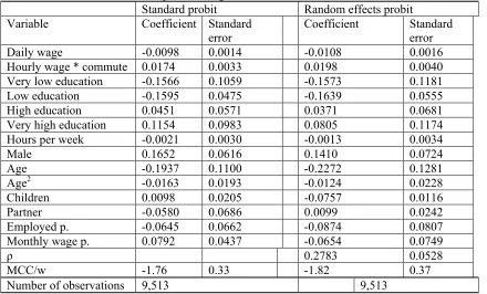
Table 5. Probit estimates of job moving

Standard probit Random effects probit Variable Coefficient Standard

error

Coefficient Standard error Daily wage -0.0098 0.0014 -0.0108 0.0016 Hourly wage * commute 0.0174 0.0033 0.0198 0.0040 Very low education -0.1566 0.1059 -0.1573 0.1181 Low education -0.1595 0.0475 -0.1639 0.0555 High education 0.0451 0.0571 0.0371 0.0681 Very high education 0.1154 0.0983 0.0805 0.1174 Hours per week -0.0021 0.0030 -0.0013 0.0034

Male 0.1652 0.0616 0.1410 0.0724

Age -0.1937 0.1100 -0.2272 0.1281

Age2 -0.0163 0.0193 -0.0124 0.0228

Children 0.0098 0.0205 -0.0757 0.0116

Partner -0.0580 0.0686 0.0099 0.0242

Employed p. -0.0645 0.0662 -0.0874 0.0807 Monthly wage p. 0.0792 0.0437 -0.0654 0.0749

ρ 0.2783 0.0528

MCC/w -1.76 0.33 -1.82 0.37

Number of observations 9,513 9,513

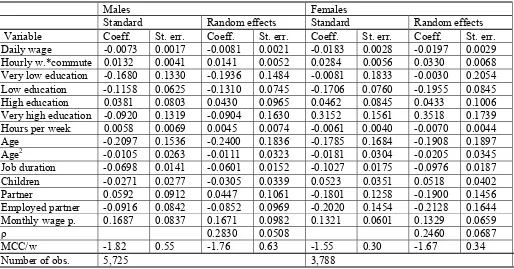
Table 6. Probit estimates of job move by gender

Males Females

Standard Random effects Standard Random effects Variable Coeff. St. err. Coeff. St. err. Coeff. St. err. Coeff. St. err.

Daily wage -0.0073 0.0017 -0.0081 0.0021 -0.0183 0.0028 -0.0197 0.0029 Hourly w.*commute 0.0132 0.0041 0.0141 0.0052 0.0284 0.0056 0.0330 0.0068 Very low education -0.1680 0.1330 -0.1936 0.1484 -0.0081 0.1833 -0.0030 0.2054 Low education -0.1158 0.0625 -0.1310 0.0745 -0.1706 0.0760 -0.1955 0.0845 High education 0.0381 0.0803 0.0430 0.0965 0.0462 0.0845 0.0433 0.1006 Very high education -0.0920 0.1319 -0.0904 0.1630 0.3152 0.1561 0.3518 0.1739 Hours per week 0.0058 0.0069 0.0045 0.0074 -0.0061 0.0040 -0.0070 0.0044 Age -0.2097 0.1536 -0.2400 0.1836 -0.1785 0.1684 -0.1908 0.1897 Age2 -0.0105 0.0263 -0.0111 0.0323 -0.0181 0.0304 -0.0205 0.0345 Job duration -0.0698 0.0141 -0.0601 0.0152 -0.1027 0.0175 -0.0976 0.0187 Children -0.0271 0.0277 -0.0305 0.0339 0.0523 0.0351 0.0518 0.0402 Partner 0.0592 0.0912 0.0447 0.1061 -0.1801 0.1258 -0.1900 0.1456 Employed partner -0.0916 0.0842 -0.0852 0.0969 -0.2020 0.1454 -0.2128 0.1644 Monthly wage p. 0.1687 0.0837 0.1671 0.0982 0.1321 0.0601 0.1329 0.0659

ρ 0.2830 0.0508 0.2460 0.0687

MCC/w -1.82 0.55 -1.76 0.63 -1.55 0.30 -1.67 0.34

Number of obs. 5,725 3,788

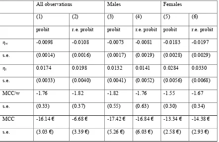
Table 7. Summary based on job moving

All observations Males Females

(1) (2) (3) (4) (5) (6)

probit r.e. probit probit r.e. probit probit r.e. probit

ηw -0.0098 -0.0108 -0.0073 -0.0081 -0.0183 -0.0197

s.e. (0.0014) (0.0016) (0.0017) (0.0019) (0.0028) (0.0029)

ηt 0.0174 0.0198 0.0132 0.0141 0.0284 0.0330

s.e. (0.0033) (0.0040) (0.0041) (0.0052) (0.0056) (0.0068)

MCC/w -1.76 -1.82 -1.82 -1.76 -1.55 -1.67

s.e. (0.33) (0.37) (0.55) (0.63) (0.30) (0.34)

MCC -16.14 € -6.68 € -17.42 € -16.84 € -13.34 € -14.38 €

s.e. (3.03 €) (3.39 €) (5.26 €) (6.03 €) (2.58 €) (2.93 €)