Munich Personal RePEc Archive
Is Deprivation Index is a vaible tool to
analyze poverty: A case study of Nepal
Bista, Chirangivi
University of Wollongong
2010
Online at
https://mpra.ub.uni-muenchen.de/28331/
Is Deprivation Index a viable tool to analyze Poverty: A case study of Nepal.
Chirangivi Bista
Abstract: This article focuses deprivation as a means of poverty and income inequality. It studies the factors explaining deprivation at the micro-level by using factor analysis technique to formulate the deprivation index and run regression to analyse key determinants of deprivation. The data is obtained from the National Living Standard Survey 2003-04. The empirical findings show that the age and gender of households head, place of residence, educational levels, occupational status, status of financial burden in a household, access to basic services and facilities are important indicators of deprivation in the Nepalese context.
1. Introduction
Poverty and inequality studies in Nepal are recent and most that exist conceptualizes poverty in absolute terms. Being land locked and infrastructure-poor, the magnitude of the poverty is not only limited to the geo-physical structures of the country. Poverty has much more to do with the socio-economic state of the locals. Female headed households, people representing the lower castes, and tribal communities are generally poor and deprived (Bajracharaya, et. al, 1999). People residing in rural areas are poor. Agriculture as the chief occupation of the majority of those populations is pervasive to chronic poverty (Bhatta and Sharma, 2006). The sector has also the lowest income multiplier effects (Devkota, 2005). Their income poverty is relatively higher compared to human poverty.
Although the monetary approach has traditionally dominated the poverty literature, the concept and methodologies of ‗deprivation‘ is an emerging tool. The measurement of deprivation to study poverty commenced from the Relative Deprivation Approach (Townsend, 1979), followed by the consensual approach of the Majority Necessity Index (Mack and Lanseley, 1985) and the Proportional Deprivation Index (Halleröd, 1994). All these approaches and measures of deprivation have broadened the scope of the concept of poverty in terms of understanding the level of deprivation and assessing individuals‘ and households‘ standards of living. Deprivation indicators are useful in addressing some of the limitations of income measures of poverty. Firstly, they aim to measure living standards directly by looking at the enforced lack of a set of material goods or social activities. Secondly, deprivation indicators are better placed to measure persistence than contemporary income. This is because the lack of items is more likely to be associated with lack of resources over a prolonged period of time.
The deprivation index, the key and emerging concept that is developed and analysed at the empirical level, is an entirely a new concept undertaken in the case of Nepal.
2. Poverty and income inequality in Nepal: a literature survey
distribution of income. Overall, a low rate of income growth, skewed income distribution, and particularly, deteriorating terms of trade of the agricultural sector vis-à-vis other sectors, have intensified poverty. GDP trends do not follow a systematic pattern of growth. The ten year long armed conflict has left the economy and society in an all-encompassing crisis (Deraniyagala, 2005).
There are many important dimensions to poverty. Based on static measurements, levels of poverty in Nepal have a strong spatial and social dimension. It is now well articulated that a high incidence of poverty prevails amongst the caste and ethnic group, women and children, rural inhabitants, and person with lower levels of income. This is evidenced by poverty literatures available both at the country specific and regional levels. As per recent poverty statistics 31per cent of the population is living below the poverty line (CBS, 2004). In rural and urban areas 35per cent of rural and 10per cent of urban people are still living below the poverty line. This poverty estimate of 43per cent rural and 22per cent urban in 1995-96 (CBS, 1996) showed a significant decline in the proportion of people living below the poverty line over time. During that period, the poverty gap ratio declined from 0.12 to 0.75, which meant that on average, poor people have moved closer to the poverty line.
Table: 1 Poverty Measures: NLSS Survey I and II
Year Head-count Index Poverty-gap1 Squared-poverty gap2
1995/96 (%)
2003/04 (%)
Change (%)
1995/96 (%)
2003/04 (%)
Change (%)
1995/96 (%)
2003/04 (%)
Change (%) Nepal 41.76 30.85 -26 11.75 7.55 -36 4.67 2.7 -42 Urban 21.55 9.55 -56 6.54 2.18 -67 2.67 0.71 -43 Rural 43.27 34.62 -20 12.14 8.50 -30 4.83 3.05 -37
Sources: CBS (2006).
A comparison of these (national) poverty figures with internationally defined poverty rates gives a more challenging state of poverty for Nepal with the rest of the world. The poverty line of US$1 results in 24.1per cent of the population being below the poverty line whereas this ratio becomes significantly higher (68.5per cent) when using US $2 as poverty line per day (World
1
Poverty gap ratio measures the mean distance below the poverty line expressed as a percentage and the mean is taken over the entire population, counting the non-poor as having zero poverty gap.
2
Bank, 2007). A comparison of quantitative and qualitative measures of poverty clearly delineates the fact that poverty is a burning problem which is subsequently declining at the later stage.
Despite a high level of poverty both in terms of incidence and severity, and as per their multiple sources of measurement, an in-depth analysis of the factors behind the decline in the level of poverty between the two survey periods shows factors such as increases in migration and remittances, diversification in agriculture - particularly the wave in commercial farming of agricultural products such as off-season vegetables, horticulture and dairy products, poultry and other animal products targeting the urban needs - to be the main reason for the improvement in the level of income in rural areas, where poverty is concentrated (NPC, 2006).
Economic inequality increased considerably over the last three decades. The Gini index—the most widely used measure of inequality—of disposable income and consumption expenditures, for example, increased from 0.30 in 1984 to over 0.38 in 1996 and to 0.47 in 2004 (CBS, 2006). The increase in income inequality observed in Nepal between 1995-96 and 2003-04 was driven primarily by the higher returns to higher education and professional and entrepreneurial skills (Wagley, 2007). The share of the top quintile on the national income and consumption expenditure increased from 40 percent in 1984 to 47 percent in 1996 and 55 percent in 2004. The latest data derived for the Gini Index is 0.37 which shows a slight decline in income inequality at present (NRB, 2008).
The planned approaches to poverty reduction also showed mixed results. Although poverty alleviation was the leading agenda item during the past three periodic plans, the achievements level has been virtually low. The percentage of poor people has not been reduced as per the targets, and although the rate of poverty declined marginally, income inequality only increased at the spatial level. There was no target available for the overall eighth plan, by the end the incidence of poverty was estimated at 42per cent, which was well behind the target in the ninth plan (38 %). The tenth plan has almost achieved its target (32 %) but there are academic debates and contradictions about this particular finding3.
3
Similarly, a key determinant of the level and intensity of both income and human poverty is access (or the lack of it) to basic social and economic infrastructure. Rural areas lack access to basic services such as education, healthcare, drinking water, roads, and access to other infrastructure and markets. Overall, the past economic reforms have completely ignored the sector (rural) where the majority of the poor reside (Cockburn, 2001).
Analysing different poverty measures-income poverty, subjective poverty line, and the human poverty index, all of them averaged around 30 per cent poverty incidence. The country's highly stubborn incidence of high poverty registered its first significant decline during 2003/04. This is considered to be the resultant outcomes of major economic reforms undertaken during the 1990s and 2000s. This has been instrumental in enhancing growth where per capita GDP growth was significantly higher and poverty rates also declined noticeably. However, the economy was not able to keep this progress for a long time.
Theoretically, growth and poverty have negative relationships. However, there may be a situation where a negative growth results in poverty reduction. This situation mostly occurs when the effect of inequality reduction on poverty supersedes the adverse impact of negative growth on poverty (Kakwani and Son, 2006). In the Nepalese contexts, the low level of GDP growth rate as well as the declining poverty levels during the latter phases of the post-reform period may be attributed to this empirical trend. However, the rate at which income inequality increases during that period does not fully comply with this growth principal.
As a whole, the key macro-economic performance both during the pre-reform4 and post-reform5 periods has been highly unfavorable in lowering a high level of poverty and inequality in the country. A higher dependence on agriculture and lower than expected growth in this sector during the post-reform period adversely affected the goal of poverty reduction in the country. The poverty alleviation initiatives show that there have been some gains in reducing poverty but several large scale problems remain to be dealt with at every level.
3. Deprivation Index
The Nepal Living Standard Surveys phase two (NLSS II) is the main data source for developing a deprivation index. This is a household level survey conducted by the Central Bureau of Statistics (CBS) Nepal during 2003-04 which follows the Living Standard Measurement Survey techniques of the World Bank. The survey utilises a two-stage stratified sampling procedure to collect data. The data is cross-sectional in nature and covers a total of 3912 households.
The key feature of the definition of deprivation that links it to the notion of poverty is its emphasis on a lack of resources as being the underlying causes of deprivation. This implies that if deprivation can be defined, it can help to identify who is in poverty and also how much income is needed to overcome it (Saunders et. al, 2008). This interpretation of the role of derivation places fewer requirements on the robustness of the deprivation indicators than if they are assumed to actually measure poverty directly (Bardasw and Finch, 2003). Thus, a substantial number of literatures confirm the fact the deprivation is a better measure to define poverty.
This study developed a deprivation index on the basis of the qualitative responses provided at the household level. They were broadly categorised into three major domains (Table: 2). First domain is related to basic needs fulfillment, second is on the status of service delivery by the state, and third domain is related to access to infrastructures and prominent facilities among the local population. All these variables are basic components that are commonly included as an
4
The pre-reform period covers the year from 1980s to 1989.
5
indicator while constructing the index. The data are organized in the form of likert scales6 interval and Cronbach‘s alpha is used for testing the reliability of the scale. Data are assigned individual weights according to their respective scale. Two procedures are used to derive a weighting of the various components of the index. One derives the weights from the data itself based on principal component analysis and the other by calculating the total deprivation index as the average score of all individual components.
The variables (components) are relevant as per their usage while developing an index of deprivation. All of them have fundamental and intrinsic significance (Klasen, 2000) and besides, they are the most important aspects representing well-being in a developing setting from the point of view of an enforced lack approach7.
While constructing the index, much more depends on the choices, the scoring, and the implicit weighting assigned to the indicators. However, for this study, it should be clearly noted that this is not an attempt to propose a definitive measure of well-being, but simply to contribute to larger debates about possible ways to capture well-being more directly than relying on several other imperfect proxies i.e. income /expenditures. The sensitivity test is conducted by constructing a core deprivation index which contains a total of thirteen components.
Two questions are central to debates concerning the measurement of poverty from a deprivation perspective: What are those standards of living whose absence indicates deprivation, and how can one decide upon the relative value of each standard of living (Sen, 1987)? The first is to determine both the deprivation measures and their respective weights according to the subjective perceptions of respondents. The second set includes the statistics obtained from factor analysis, which is a technique of identifying underlying dimensions of variation on which the observed variables are loading by means of various extraction and rotation methods (Tabachnick and
6
Each indicator is scored on a scale of 1 to 3 to roughly ensure that a score of three represents a best possible condition or standard; two gives the moderate level whereas the score of one gives low level of standard or deprivation.
7
Fidell, 2001).
The decision regarding the number of factors depends more on the nature of the survey data. Nevertheless, Eigenvalues representing variance or the screen test of Eigenvalues plotted against factors can aid this decision. The latter was used in this study to determine the number of factors trialed. After several trials, a three factor solution obtained through combining principal components analysis with a varimax rotation technique (orthogonal) was extracted. In fact, this particular solution did not prove significantly different from those produced by other combinations.
The ultimate aim in conducting factor analysis is to explore how variables are correlated with each other, and how they can be summarised to avoid any risk of repetition. The principal components extraction technique is deemed more suitable for this purpose than testing a hypothesis about underlying processes (Tabachnick and Fidell, 2001). Additionally, the varimax rotation technique, which maximises variance of factor loadings, was preferred to increase the sensitivity of the weights to the perceptions of the minority.
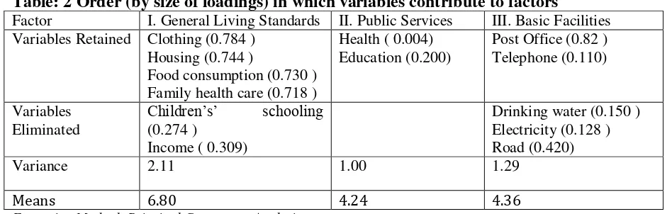
The decisions relating to the selection of variables to be interpreted by each factor, or to be retained within the index, were based on the factor loading scores of the individual variables on it. Factor loading scores indicate the weights used in determining the unique contribution of each factor to the variance in a variable. In solutions using orthogonal rotation they also refer to the correlations between variables and factors. As a principle ( a rule of thumb), the cut-off point is set at 0.30, as a result of which some items relating to living standard and facilities are eliminated.
The respondents seem more inclined to conceive deprivation in terms of a lack of living standard pertaining to a fulfillment of basic needs. The significance of each factor was established by looking at the percentage of variation explained by it. As shown in Table: 2, three factors proved almost equally significant in terms of the amount of variance they explained. However, the distribution of their total means seemed to indicate a slight order to the way in which each dimension was valued; the general living standard came first, basic facilities second, and public services last. This may suggest that respondents are rather rational in their judgments as to how these dimensions/ necessities should be prioritised.
[image:10.612.78.552.341.492.2]These results are reliable on two grounds. Firstly, the factor solutions obtained from numerous trials proved rather stable across different extraction and rotation methods8. Secondly, the variables meaningfully loaded on to each extracted factor.
Table: 2 Order (by size of loadings) in which variables contribute to factors
Factor I. General Living Standards II. Public Services III. Basic Facilities Variables Retained Clothing (0.784 )
Housing (0.744 )
Food consumption (0.730 ) Family health care (0.718 )
Health ( 0.004) Education (0.200)
Post Office (0.82 ) Telephone (0.110)
Variables Eliminated
Children‘s‘ schooling
(0.274 )
Income ( 0.309)
Drinking water (0.150 ) Electricity (0.128 ) Road (0.420)
Variance 2.11 1.00 1.29
Means 6.80 4.24 4.36
Extraction Method: Principal Component Analysis Rotation Method: Varimax
Figure in the parenthesis are the respective weights.
In the process of factor analysis, one useful comparison is to examine the correlation between the deprivation index and its various components (Appendix Table: 2). Here, all components are positively (significantly) correlated with the deprivation score and most components are closely and positively correlated with each other. At the same time the strengths of the correlation differs considerably.
8
Similarly, to validate the results of this analysis, a split-half validation was conducted to ensure the stability and generalisation of the model. While the communalities differ for two models, in all cases they are above 0.50, indicating that the factor model is explaining more than half variance in all of the original variables.
For the multi-variates analysis of the determinant of poverty, two distinct and alternative approaches of econometric tools were used in the study. These are the deprivation index and income regression model. Detailed methodology for the study follows the empirical studies of Ravillion (1996) and Deaton (1997). The regression analysis was conducted to study the level of deprivation with a host of explanatory variables at the household level. A subsequent income regression was performed to enable a comparative study on the determinants of poverty between the level of deprivation and income. First, an attempt to analyse the deprivation index was based on significant numbers of quantitative and qualitative variables. Henceforth, the focus was entrusted mainly to household level deprivation represented by the first model here.
Deprivation Index
i i i
DI
X
D
(i)
Income Regression
ln i i
i
i
W
X
D
(ii)Where as,
DI is Deprivation Index
lnWi is natural log of nominal per capita income divided by the national poverty line β is parameter of the exogenous variables.
Xi is the set of exogenous household characteristics or determinants of poverty Di is dummy variables
is random error term
dependent variable in this line was the Income Regression Model based on normalised indicators derived as the natural log of per capita income divided by the national poverty line. However, the explanatory variables for both models were the same (Appendix Table: 3). Here, the objective was to analyse the deprivation index amongst different explanatory variables identified at the household levels and seek for its correlation with a host of explanatory variables.
The choices of the explanatory variable for analysing key determinants of poverty was based on the empirical application of the variables and the findings of relevant developing country studies, (Lanjouw and Ravallion, 1995; Deaton and Paxton, 1998). These variables ranged from household demographics to different other socio-economic and physical characteristics because they were considered to be important determinants of deprivation and or poverty. Similarly, the selection of explanatory variables for the model was also influenced by the National Living Standards specific survey studies that was recently conducted in developing countries like Sri Lanka (De Silva, 2008), Bangladesh (Kotikula, et. al 2007), Mozambique (IFPRI, 2000) and South Africa (Klasen, 2000) etc.
Most of the variables possess both the expected signs and the appropriate coefficients while explaining the level of deprivation for Nepal. The size of the coefficients associated with these regressors varies accordingly. The key explanatory variables for the deprivation index are the age of the households, sex of the households, access to drinking water, access to toilet, access to (basic) facilities, household location characteristics (rural/urban), educational level, and occupation of head of households, status of livestock ownership and financial burdens of the household. These are the most common factors strongly associated with deprivation/poverty. This is further evidenced by the empirical findings of the ongoing literatures on deprivation and poverty. The regressors constitute of both the quantitative and qualitative variables.
Households who have access to potable drinking water facilities are likely to be deprived as low as by 0.43per cent. Similarly, sanitation as an indicator of deprivation/poverty has its own significance and elementary values with its impact on health and maintaining a general living standard. Households with sanitation facilities, i.e. toilets, are completely non-deprived.
The educational attainment of the head of household is an important indicator of deprivation/poverty. Both the primary and secondary levels of education are extremely important, as depicted by its appropriate coefficients and highly significant variable. Households who do not have up to primary (0.54 %) and secondary/tertiary levels of education (0.79 %) are likely to be highly deprived. Here, by holding other variables constant, the role of tertiary education is deemed vital in explaining the increasing level of deprivation at the households level.
There is a positive association between the level and degree of financial burden a household is in, and poverty. A poor household is usually in debt because it is assumed there will always be a financial scarcity so they rely on several formal and informal financial sources for debt. Other factors remaining constant, among those households who do not have any types of financial burden, their level of deprivation decreases significantly (0.82 %).
The livestock ownership status by a household is an important determinant of deprivation/poverty. The larger the number of livestock a household possesses, the lower the likelihood of being in poverty. By holding all other variables constant, households with livestock holdings envisage that the deprivation index decreases by as low as 0.51per cent.
A comparison of the coefficients associated with the deprivation index and income regression models (Table: 3) gives a more vivid picture of the determinants of poverty from two different viable aspect. In the regression analysis the dependent variable is frequently influenced by the qualitative variables as well. Here, the major influential nominal scale variables are sex, geographical regions, housing characteristics, occupation and education. In both the models, the assessment of overall sign and magnitude of the coefficients depict that the deprivation index model is much better at explaining the key determinates of poverty and/or deprivation than the income regression model. Although the majority of coefficients are significant in the income regression model, their power and degree of explaining the variability by their respective coefficients are much low than the deprivation index.
Both regression analyses depicted a low level of R2 i.e. the coefficient of determination explains only about 15per cent variations in the deprivation index. In the regression analysis, literatures show that such a low R2 value (0.14678) is typically observed in cross-sectional data with a large number of observations (Gujarati, 2003). Apparently, a low R2 value can also be statistically significant (i.e. different from zero). In the given model also, the R2 value is statistically significant, since the computed F value of about 37.20 is highly significant, as its p value is almost zero i.e. the F statistics tests the hypothesis that all the slope coefficients are simultaneously zero; that is, all the explanatory variables jointly have no impact on the regressand.
Table: 3 Test Statistics of Deprivation Index and Income Regression
Variable
Coefficients
Deprivation Index Income Regression
C -0.787144 (0.521910) -0.237632 (0.190350) AGEHHH 0.071718** (0.021028) 0.038371*** (0.007669) ASQR -0.000693** (0.000215) -0.000388*** (7.830000) HHSIZE -0.058720 (0.048772) -0.162312*** (0.017788) HSQR 0.004401 (0.002859) 0.005495 (0.001042) AGRILABOUR -0.180403 (0.135016) -0.145261 (0.049253) DW 0.427252*** (0.107345) 0.229474*** (0.039155) GEOLOC -0.742068*** (0.146210) -0.202679*** (0.053350) LAND 0.320151 (0.137433) 0.182346** (0.050136) LIVESTOCK -0.508025*** (0.149971) 0.303390*** (0.054708) LOAN -0.821769*** (0.110066) -0.167992*** (0.040144) PROFESSIONALS 0.173448 (0.323057) 0.158273 (0.117842) PRIMARY 0.543626** (0.198546) 0.044120 (0.072401) TERTIARY 0.761990 (0.468472) 0.254137 (0.172611) SEXHHH -0.021881*** (0.129560) -0.262533*** (0.047269) TOILET 1.034323*** (0.117778) 0.555598*** (0.042955) ETHN -0.014014 (0.141243) 0.084706 (0.051544) ADR 0.034647 (0.165598) -0.249427*** (0.060404) ATF -0.042217*** (0.004312) 0.007383*** (0.001572)
R-squared 0.146787 0.159223
Adjusted R-squared 0.142842 0.155331
S.E. of regression 3.093536 1.128032
Sum squared resid 37255.87 4948.581
Log likelihood -9959.244 -6006.503
F-statistic 37.20854 40.91562
Prob(F-statistic) 0.000000 0.000000
Mean dependent var -1.82E-05 0.229460
S.D. dependent var 3.341372 1.227377
Akaike info criterion 5.101352 3.083676
Schwarz criterion 5.131813 3.114163
Hannan-Quinn criter. 5.112162 3.094496
Durbin-Watson stat 1.669038 1.860097
N 3912 3908
Notes: Figures in the parenthesis are standard errors.
4. Discussion
The time series analysis on the incidence of poverty in Nepal demonstrates that levels of poverty were lower in post-reform (31 %), vis-à-vis pre-reform (42 %) periods. In terms of validating this poverty rate, even after applying a series of different poverty measures, it also results in the same rate of poverty incidence at the national level. Income inequality shows opposite trends. Gini coefficients based on per capita income increased from 0.24 points during the pre-reform period to 0.37 at the present post-reform period. The level of differences in inequality in urban areas is significantly higher than rural areas.
The deprivation index is envisioned in the form of a lack of living standards pertaining to the fulfillment of basic needs because the nature of poverty/deprivation for the country still revolves within this periphery. This implies that the poverty level is still comparatively higher with its absolute and chronic in nature. The poverty profiles drawn here, supplemented by the multi-variate analysis of poverty determinants, identify the household and location/geographic attributes most closely associated with deprivation. The key proximate determinants of poverty are age and sex of the head of households, place of residence, lack of access to basic amenities and services, livestock ownership status, status of financial burden in the households, level of education, professions, and access to basic services and facilities.
As an alternative to calculating the total deprivation index based on the average score of all individual components, a rough estimate gives a 48per cent deprivation level for the country as a whole. This is successively higher than the present incidence of poverty of 31per cent. This can be the initial evidence to prove that the level of deprivation in Nepal is generally high and very profound.
There are many different approaches to the measurement of deprivation. As per their purpose, the deprivation indices combine several observations from a variety of domains into a single variable. Therefore, the deprivation index and comprehensive social and economic indicators should not be seen as alternatives, but as two complementary elements in developing more effective policies to target poverty and exclusion at local levels.
5. Conclusion
Nepalese poverty/deprivation level is still dominated by the basic necessities of life. People still prioritise food, shelter and clothing as vital for maintaining their general living standards. Their perception and conceptualisation of poverty is very conventional. A large part of the population is still engulfed in a vicious circle of poverty, which clearly indicates this widespread poverty problem. Ultimately, the incidence poverty is of an absolute and chronic nature.
The concept and measurement of poverty, inequality, and income vary widely according to the methodology adopted by the survey, making data inconsistent. This is clearly shown by empirical studies of poverty.
Poverty profiles in Nepal are an outcome of surveys carried out at different points of time. Due to the methodological variations, they are not directly comparable. So far, only two waves of cross sectional data are available to measure poverty which places limits on an in-depth study so this deprivation study may provide further impetus to the ongoing poverty literature in the country.
The studies on income distribution also revealed a large inter-survey variation. This was also due to the treatment of income in terms of household income in one survey and per capita income in another. As households with higher levels of income also tend to have smaller families, the distribution of income on a per capita basis tends to be more even than on a household basis.
on the factor analysis (score).The deprivation indicator was assumed to be summary statistics of overall living standards, not as key indicators in their own right of specific dimensions of poverty. However, what is important in the factor analytical approach is the degree to which indicators correlate to each other and to the unobservable underlying characteristics that we wish to measure, which is generalised deprivation. Deprivation indicators do not stand alone in their own right as measures of specific aspects of poverty, but represent a ‗proxy‘ for overall deprivation.
This research is based on secondary sources of data; there might be some drawbacks regarding sample size pre-specified objectives and toward an attempt to re-utilise it. While growth is relatively easy to define and quantify, the concept of poverty is multi-dimensional and complex. Measurements of poverty based on income and expenditure are clearly inadequate. The concept needs to be broadened to include an array of social indicators.
In the absence of chronological (time series) data on poverty and income inequality, a poverty profile may fill the gap and act as a descriptive tool for giving clues to the underlying determinants of poverty. The post reform was associated with a widening income gap among that rural-urban population. Income inequality is substantially higher in urban areas. On the contrary, poverty is significant in rural areas. This also points towards a higher level of deprivation amongst rural populations. So, this interesting but compelling nexus between deprivation/poverty and inequality can become a viable area of study for further exploring and understanding deprivation/poverty dynamics.
Appendices
Appendix Table: 1 Components of Subjective Measure of Deprivation
Component (Frequency)
Score (1 signifying most deprived, 3 least)
1 2 3
Basic needs fulfillment
Food consumption 1120 2713 79
Housing 1477 2405 30
Clothing 1256 2625 31
Family Health care 1030 2846 36
Children‘s Schooling 803 2269 840
Income 2523 1345 44
Service delivery status
Health services 817 2436 659
Education services 419 1981 1512
Access to Infrastructure
Drinking water 715 1547 1650
Electricity 285 1106 2521
Road 1520 1639 753
Post office 463 2240 1209
Telephone 760 1741 1411
Total Responses 3912
Source: Derived from NLSS-II Survey, 2004.
Appendix Table: 2 Correlation Coefficient between Deprivation Index and its components
DI FC Housing Clothing FHC Health Education Post office
Tele phone
DI 1
FC 0.550** 1.000
Housing 0.604** 0.412** 1.000
Clothing 0.600** 0.471** 0.477** 1.000
FHC 0.568** 0.347** 0.424** 0.442** 1.000
Health 0.511** 0.044** 0.093** 0.080** 0.104** 1.000 Education 0.512** 0.026 0.062** 0.054** 0.035* 0.269** 1.000 Post office 0.417** 0.064** 0.100** 0.074** 0.092** 0.179** 0.216** 1.000 Telephone 0.347** 0.002 0.034* 0.008 0.046** 0.111** 0.152** 0.414** 1.000 ** Correlation is significant at the 0.01 level (2-tailed).
Appendix Table: 3 List of Variables for Regression Analysis
Variables Definitions Symbol Mean S.E. Type Dependent Variables
Deprivation Index Subjective Deprivation Index DI 0.0 3.341 Income Poverty Normalized poverty line income lnWi 9.08 2.237 Explanatory Variables
Household size HSIZE 5.504 2.639 C
Household size square HSQR 2271.48 1390.85 C Age of Household head
(years)
AGEH
45.488 14.226 C
Age Square ASQR 37.256 43.689 C
Age Dependency Ratio per cent of family member below 15 and above 65 years in the household
ADR
0.467 0.313 C
Access to Facilities (in hours)
Average time spend to reach basic facilities and infrastructures.
ATF
3.098 11.790 C
Education of Household head (Primary)
= 1 If household head has primary level of education =0 otherwise
PRIMARY
0.067 0.251
D1
Education of Household head (Secondary)
= 1 If household head has secondary level of education =0 otherwise
SECONDA RY
0.043 0.204 R
Education of Household head (Tertiary)
= 1 If household head has tertiary level of education =0 otherwise
TERTIARY
0.012 0.108
D2
Sex of Household head = 1 If household head is female =0 otherwise
SEXHH
0.192 0.394
D3
Area of Residence (Rural/Urban)
= 1 If the household is Rural =0 otherwise
GEOLOC
0.721 0.449
D4
Land holdings status = 1 If household owns land =0 otherwise
LAND
0.726 0.446
D5
State of Financial Burden = 1 If household is in debt =0 other wise
LOAN
0.649 0.477
D6
Sources of Drinking Water = 1 If household has access to potable drinking water
=0 other wise
DW
0.498 0.500
D7
Livestock ownership status = 1 If household owns livestock =0 other wise
LIVESTOC
0.730 0.444
D8
Toilet facilities = 1 If household has own toilet facility
=0 other wise
TOILET
0.460 0.498
D9
Occupation specific(1) = 1 If household main occupation is service
=0 Otherwise
SERVICE
0.038 0.190 R
Occupation specific(2) = 1 If household is in professionals and experts jobs =0 Otherwise
PROFESSI ONAL
0.027 0.163
D10
Occupation specific(3) = 1 If household is involved in agriculture/labour
=0 Otherwise
AGRILABO UR
0.794 0.405
D11
Ethnicity = 1 If household is of deprived/disadvantage groups =0 other wise
ETHN
0.847 0.360
D12
References
Bahtta, S. and Sharma, S. (2006). ‗The Determinants and Consequences of Chronic and Transient Poverty in Nepal‘ CPRC Working Paper (66), UIC/TU.
Bajracharya, B. B., Suman S. and Osmani, S. (1999). ‗Assessment of National Anti Poverty Programmes‘: The Case of Nepal. Kathmandu: UNDP.
Bardasw, J. and Finch, N. (2003). ‗Overlaps in Dimensions of Poverty‘. Journal of Social Policy, 32 (4), 513-525.
CBS (1996). ‗Nepal Living Standards Survey Report 1996-97‘. Main findings. Central Bureau of Statistics. National Planning Commission, Kathmandu.
CBS (2004). ‗Nepal Living Standards Survey 2003-04‘. Statistical Report. Central Bureau of Statistics. Kathmandu.
CBS (2006). ‗Resilience Amidst Conflict‘- An Assessment of Poverty in Nepal, 1995-96 and 2003-04. ADB, DFID and WB.
Cockburn, J. (2001). ―Trade Liberalization and Poverty in Nepal: A Computable General Equilibrium Micro simulation Analysis‖, Discussion Paper 01 (18), CREFA, University Laval.
Deaton, A. (1997), The Analysis of Household Surveys: A Microeconometric Approach to Development Policy, Johns Hopkins University Press for the World Bank, Baltimore.
Deaton, A, and Paxton, C. (1998). ‗Economies of Scale, Household Size, and the Demand for Food. J.P.E. (106): 897-930.
De Silva, I. (2008). ‗Micro-level determinants of poverty reduction in Srilanka: A Multivariate Approach‘, Department of Economics, Texas Tech University, USA.
Deraniyagala, S. (2005) ‗The political economy of civil conflict in Nepal.‘ Oxford Development Studies 33(1), 47–62.
Devkota. S. R. (2005). ‗The Politics of Poverty Alleviation in Nepal: Structural Analysis of Socioeconomic Development from the Past Five Decades‘. Heidelberg Papers in South Asia and Comparative Politics; Working Paper (25).
Geda, A., Jong, N., Kimenyi, M. S. and Mwabu, G. (2005). ‗Determinants of Poverty in Kenya: A Household level Analysis‘ University of Connecticut, Departments of Economics Working Paper Series.
Gujarati, D. (2003). ‗Basic Econometrics‘, Fourth Edition. New York: McGraw-Hill.
Research Centre Discussion Paper (50), University of New South Wales, Sydney.
IFPRI (2000). ‗Determinants of Poverty in Mozambique: 1996-1997.‘ Food Consumption and Nutrition Division. Washington D.C.
Kakwani, N. and Son, H. (2006). ‗Pro-Poor Growth: The Asian Experience‘. UNU, Research Paper (56).
Klasen, S. (2000). ‗Measuring Poverty and Deprivation in South Africa‘, Review of Income and Wealth Series 46, (1), March 2000.
Kotikula, A., Zamam, H. and Narayan, A. (2007). ‗Explaining Poverty Reduction in the 2000s: An analysis of the Bangladesh Household Income and Expenditure Survey.‘ South Asia Region, World Bank.
Lanjouw, P. and Ravallion, M. (1995), ‗Poverty and Household Size‘, Economic Journal, Vol. 105 pp.433.
Mack, J. and Lansley, S. (1985). ‗Poor Britain‘ (George Allen and Unwin, London).
NPC (2006). ‗An Assessment of The Tenth Plan: Poverty Reduction Strategy Paper 2002-2007, Fourth Progress Report‘, Kathmandu, Nepal.
NRB (2008). ‗Household Budget Survey Nepal: 2005- 2006.‘ Nepal Rastra Bank, Kathmandu, Nepal.
Ravallion, M.(1996). ‗Issues in Measuring and Modelling Poverty‘. The Economic Journal, (106), 1328-1343.
Saunders, P., Hill, T. and Bradbury, B. (2008) ‗Poverty in Australia: Sensitivity Analysis and Recent Trends.‘ ACOSS, SPRC Report (4/08).
Sen, A.K. (1987). ‗The Standard of Living‘. Cambridge University Press, Cambridge.
Tabachnik, B.G. and Fidell, L. S. (2001), ‗Using Multivariate Statistics‘ 4th edition. (Allyn and Bacon, Boston).
Townsend, P. (1979). ‗Poverty in the United Kingdom: A Survey of Household Resources and Standards of Living‘. Penguin Books, Harmondsworth.
Wagle, R. U. (2006). ‗Economic Inequality in Kathmandu: A Multi-Indicator Perspective‘. Himalayan Journal of Development and Democracy, 1(1), 1-30.