A note on GDP now /forecasting with dynamic versus static factor models along a business cycle

(1)

Munich Personal RePEc Archive

A note on GDP now-/forecasting with

dynamic versus static factor models

along a business cycle

Buss, Ginters

Central Statistical Bureau of Latvia, Riga Technical University

16 April 2010

Online at

https://mpra.ub.uni-muenchen.de/22147/

(2)

A note on GDP now-/forecasting with dynamic

versus static factor models along a business cycle

∗

Ginters Buss

†

Riga Technical University

and

Central Statistical Bureau of Latvia

April 16, 2010

Abstract

We build a small-scale factor model for the GDP of one of the hard-est hit economies during the lathard-est recession to study the exact dynamic versus static factor model performance along a business cycle, with an emphasis placing on nowcasting performance during a pronounced switch of business cycle phases due to the latest recession. We compare the factor models’ nowcasting performance to a random walk, autoregressive and the best-performing nowcasting models at our hands, which are vec-tor auvec-toregressive (VAR) models. It is shown that a small-scale static factor-augmented VAR (FAVAR) model tends to improve upon the now-casting performance of the VAR models when the model span and the nowcasting period stretch beyond a single business cycle phase, while ex-act dynamic fex-actor models tend to fail to detect the timing and depth of the recession regardless of ARMA specifications. As regards the case when the model span and the nowcasting period are contained within a single business cycle phase, static and dynamic factor models appear to show similar performance with potentially slight superiority of dynamic factor models if the factor-forming set of variables and factor dynamics are carefully selected.

Keywords: nowcasting, business cycle, static versus dynamic factors, small-scale FAVAR, VAR, GDP

JEL code: C22, C32, C44, C52, C53

∗_{Acknowledgments: This work has been supported by the European Social Fund within} the project “Support for the implementation of doctoral studies at Riga Technical University”. The author would like to thank his supervisor Viktors Ajevskis for his guidance. Remaining errors are the author’s own. The opinions expressed in this paper are those of the author and do not necessarily reflect the views of the Central Statistical Bureau of Latvia.

(3)

1 Introduction

The choice between static and dynamic factors in now-/forecasting GDP is un-resolved. Some papers find dynamic factors superior over the static ones (see, for example, den Reijer (2005)). Other papers find little or no advantage of dynamic over static factors. For example, Schumacher (2005) finds that dy-namic factors only slightly outperform static factors. D’Agostino and Giannone (2007) find static and dynamic factors perform similarly. Marcellino and Schu-macher (2008), among other results, report that information content of now- and forecasts hardly change if factors are estimated by static rather than dynamic principal components analysis. Ajevskis and Davidsons (2008) also find simi-lar performance between static and dynamic factors. Finally, there are papers that argue for static over dynamic factors. For example, Boivin and Ng (2005) state that static factors are easier to construct than dynamic factors, and are favored on practical grounds. This paper contributes to the now-/forecasting literature by comparing GDP nowcasting performance of dynamic versus static factor models along a business cycle. For the fulfillment of the task, we had to choose the size of factor-forming set of variables, i.e., we had to decide whether to use a large-scale or a small-scale factor model, and what data to use.

Regarding the choice between large-scale and small-scale factor models, the following empirical evidence is observed. First, several papers on large-scale factor models compare the models only to simple benchmarks, instead of the best-performing models, and find large-scale factor models superior. For exam-ple, Siliverstovs and Kholodilin (2010) use a large-scale approximate dynamic factor model from 562 indicators and compare its now-/forecasting performance to, what they call, a naive constant-growth model, and find the factor model being superior. As another example, Ajevskis and Davidsons (2008) use large-scale static and approximate dynamic factor models from 126 indicators, com-pare them to a benchmark autoregressive model, and find factor models tending to be superior over the benchmark. There is another kind of papers that finds that large-scale factor models can not improve GDP now-/forecasting compared to non-factor models. For example, Banerjee, Marcellino and Masten (2010), inter alia, forecast the industrial production in Germany, and find that large-scale factor models extracted from 90 monthly series can not improve upon the forecasting performance of a simple autoregressive model, and conclude that factors per se may not increase the forecasting precision of models. Likewise, Gupta and Kabundi (2008, 2009) although have a misleading abstract, find that a large-scale factor model performs worse than a vector autoregressive model in forecasting South Africa’s GDP. Finally, there are papers that argue for small-scale over the large-small-scale factor models (see, for example, Schneider and Spitzer (2004), Boivin and Ng (2003)). Given the lack of empirical evidence or rationale for clear advantage of large-scale over small-scale factor models in GDP now-/forecasting, our choice falls to using parsimonious, small-scale factor models.

(4)

the paper might be repeated on any data with a pronounced switch of business cycle phases, including generated data. Considerations of using other data are left for further research.

Note that this paper does not discuss the now-/forecasting performance of Markov-switching factor models (see, among others, Kim and Yoo (1995), Chau-vet (1998), Kim and Nelson (1998), ChauChau-vet and Hamilton (2005), and Cama-cho, Perez-Quiros and Poncela (2010)).

The paper is organized as follows. Section 2 describes the methodology of factor models and their estimation. Section 3 presents the results for the now-casting performance of static, dynamic and mixed factor models versus a random walk (RW), autoregressive (AR), and vector autoregressive (VAR) models dur-ing a smooth growth phase as well as durdur-ing a pronounced switch of business cycle phases. Finally, Section 4 concludes.

2 Methodology

This section discusses the estimation of static and exact dynamic factors, and is mainly in line with Doz and Lenglart (1999) and Dubois and Michaux (2010).

Consider an (n + 1)-dimensional vector autoregressive model of order r, VAR(r):

     yt

x1t

.. . xnt      =     

a0+a01yt−1+· · ·+a0ryt−r+· · ·+a011x1,t−1+· · ·+a0nrxn,t−r+u0t

a1+a11yt−1+· · ·+a1ryt−r+· · ·+a111x1,t−1+· · ·+a1nrxn,t−r+u1t

.. .

an+an1yt−1+· · ·+anryt−r+· · ·+an11x1,t−1+· · ·+annrxn,t−r+unt      , (1) whereytis a scalar dependent variable at timet= 1, . . . , T,xt= (x1t, . . . , xnt)′

is ann×1 vector of endogenous explanatory variables at timet,ut= (u0t, . . . , unt)′

is an (n+ 1)×1 vector of innovation processes at time t with E(ut) = 0,

E(utu′t) = Σu, E(utu′s) = 0 for s 6= t and t = 1,2, . . .. If n is large, model

(1) incurs in a curse-of-dimensionality problem. A cure for this problem is to use a relatively small number of factors that are weighted averages of the pre-dictors. We will consider two types of factor extractions - static and exact dynamic. Static factors are obtained`a la Stock and Watson (1998) as follows. It is assumed that xt can be represented as

xt= ΛFt+et, (2)

whereFtis ak×1 vector of common factors at timet, Λ is ann×kmatrix of

factor loadings, andet is ann×1 vector of white noise processes at time t. It

is assumed that

E(yt+1|Ft, xt, yt, Ft−1, xt−1, yt−1, . . .) =E(yt+1|Ft, yt, Ft−1, yt−1, . . .). (3)

The assumption in (3) permits the dimension reduction of the matrix of explana-tory variables fromntok. Ftis obtained by principal components analysis, i.e.,

by selecting k eigenvectorsνj, j = 1,2, . . . , k (that are of unit length) ofx′x,

where x = (x1, . . . , xT)′, associated with the largest k eigenvalues of x′x and

projecting xon the eigenvectors, Fj =xνj, j = 1,2, . . . , k; Ft then is the tth

(5)

The dynamic factor model is estimated as in Doz and Lenglart (1999), that develops an exact dynamic factor model, where factors are extracted from a relatively small number of variables. The procedure is described as follows. If

nis the number of the variables under study,T the number of observations for each variable,xitthe value taken by thexivariable at timet, and ifF1, . . . , Fk,

k < nare the unobservable factors, the model has the following form:

xit=λi1F1t+· · ·+λikFkt+uit

fori= 1, . . . , n and for allt. Each common factorFj contributes to the

expla-nation of the xi variable with a loading equal toλij. The idiosyncratic terms

(uit)t∈Z are assumed to be independent of each other and independent of the

common factors:

E(uitujs) = 0∀i6=j, ∀(t, s)

E(uitFjs) = 0∀(i, j), ∀(t, s).

In the model designed for individual data, the common and idiosyncratic factors are assumed to be white noises, i.e.,

E(uituis) = 0∀i,∀t6=s

E(FitFis) = 0.

The model designed for individual data cannot be directly applied to time series, which generally show temporal autocorrelations. For this reason, it is called a static factor model. Using matrix notations

xt= (x1t, . . . , xnt)′, Ft= (F1t, . . . , Fkt)′

ut= (u1t, . . . , unt)′,Λ = (λij)1≤i≤n

1≤j≤k,

this model can be written as follows:

xt= ΛFt+ut,

where

E(Ft) = 0

E(ut) = 0

E(utu′t) =D=diag(d1, . . . , dn)

E(Ftu′s) = 0, ∀(t, s), t6=s

E(utu′s) = 0, ∀(t, s), t6=s.

It is easy to see that the common factors are only defined up to a linear transfor-mation, that is, it is always possible to premultiplyFtby any invertible matrix,

as soon as Λ is postmultiplied by the inverse of the same matrix. Generally, it is assumed that V ar(Ft) = Ik, so that Ft and Λ are defined up to a

rota-tion matrix (at the estimarota-tion stage, they are fixed by imposing supplementary identifying constraints; see below). If it is imposed thatV ar(Ft) =Ik, then

(6)

such that

V ar(xit) = k X

j=1

λ2ij+di, i= 1, . . . , n.

Eachλ2ij represents the part ofx ′

is variance which is explained byFj; thus,h2i = Pk

j=1λ2ijrepresents the total contribution of the factors tox ′

is variance. On the

other hand,V ar(ui) =di is the part ofx′is variance which is not explained by

the common factors.

There are two main methods to estimate the static model: principal com-ponents analysis (PCA) and the Maximum Likelihood (ML) under a Gaussian hypothesis. The first one does not need to make preliminary assumption about the number of factors, while this is necessary for the ML estimation. On the other hand, the ML gives efficient estimates of the parameters, which is not the case for PCA. Both methods are implemented as follows. At the first stage, the PCA is performed. Then, the ML estimation is run for the the appropriately chosen number of factors. Since we consider exact factor models, it is assumed that the processes (uit) are uncorrelated with each other at all leads and lags.

In this dynamic framework, the likelihood under the Gaussian assumption is not equal to the static model’s likelihood. However, Doz and Lenglart (1999) show that, in a stationary framework, the estimators obtained by the maximization of the static model’s likelihood are consistent estimators of the parameters. In brief, it is supposed that each of the real processes (Fit) and (uit) is weakly

sta-tionary and can be autocorrelated, but that the model is estimated by a standard ML procedure as if those processes were Gaussian and were not autocorrelated. The stationarity of the processes (Fit) and (uit) implies that the process (xt)

is stationary as well. The parameters of the model can be written in a vector

µ = (vecΛ′

, d′₎′_,where

d= (d1, . . . , dn)′. The estimator ˆµT, which is obtained

this way is then an M-estimator of µ. Doz and Lenglart (1999) show that this estimator is consistent. Shortly, denote zit =xit−x¯i and zt = (z1t, . . . , znt)′

for any t, S = 1

T P

tztzt′ the empirical covariance matrix of the observations

and Σ = ΛΛ′₊_D _{the theoretical covariance matrix. The quasi-likelihood of the}

model is computed under the Gaussian assumption as if neither the factors, nor the idiosyncratic components were autocorrelated. Up to a constant term, the quasi-likelihood can be written as

LT(z, µ) =

1

T

T X

t=1

lnIt(z, µ)

=−1

2ln(det(ΛΛ

′

+D))−1

2tr((ΛΛ

′

+D)−1_S₎

Letµ0be the true value of the parameterµ. It is assumed thatµbelongs to a set

of the formRnk_×_[_α,₊_∞₎n_,_{α >}_{0, which contains}_µ

0. Under this assumption, Σ

is an invertible matrix, so the quasi-likelihood is well defined. The proof that the M-estimator ˆµT, that maximizesLT(z, µ), is consistent, relies on several steps.

First, Doz and Lenglart (1999) show that, in order to maximize the function on

Rnk_×_[_α,₊_∞₎n_{, it is sufficient to maximize the function on a compact subset}

ofRnp_×_[_α,₊_∞₎n_{. Then, they show that the function has properties which are}

sufficient to ensure the consistency.

(7)

com-ponents following an AR(l) process can be written as

xit=mi+λi1F1t+. . .+λikFkt+uit

(1−φj1L−. . .−φjpLp)Fjt = (1−θj1L−. . .−θjqLq)ǫjt

(1−ρi1L−. . .−ρilLl)uit=ξit (4)

fori= 1, . . . , n,j= 1, . . . , kand for allt, where ǫjt andξit are the innovations

ofFtand uit at time t,l is the order of the AR process governinguit, and the

processes (ǫjt) and (ξit) are mutually independent. For identification purposes,

the variance of the factor idiosyncratic components,ǫjt, is set to take the value

0.25.

Model (4) can be put into the state-space representation

xt=Zαt+et (5)

αt=Aαt−1+Rηt, (6)

where the processes (et) and (ηt) are serially uncorrelated and mutually

uncor-related at all leads and lags, and

E(et) = 0

V ar(et) =H

E(ηt) = 0

V ar(ηt) =Q.

In our case, the state-space form of the model, (5) and (6), is the following:

xt=

Λ 0n×k(p+q−1) In 0n×n(l−1)

                 Ft .. .

Ft−p+1

ǫt

.. .

ǫt−q+1

ut

.. .

ut−l+1

(8)

                 Ft .. .

Ft−p+1

ǫt

.. .

ǫt−q+1

ut

.. .

ut−l+1

                 =        

φ θ 0k×nl

Ik(p−1)×kp 0k(p−1)×kq 0k(p−1)×nl

0k×kp 0k×kq 0k×nl

0k(q−1)×kp Ik(q−1)×kq 0k(q−1)×nl

0n×kp 0n×kq ρ

0n(l−1)×kp 0n(l−1)×kq In(l−1)×nl                         

Ft−1

.. .

Ft−p

ǫt−1

.. .

ǫt−q

ut−1

.. .

ut−l                  +         Ik

0k(p−1)×k 0k(p+1)×n

Ik

0k(q−1)×n

0[k(q−1)+nl]×k In

0n(l−1)×n         ǫt ξt , where

xt= 

 

x1t

.. .

xnt 



 Λ =



 

λ11 · · · λ1k

..

. ... ...

λn1 · · · λnk 



 Ft=



 

F1t

.. .

Fkt 



 ǫt=



 

ǫ1t

.. . ǫkt   

ut= 

 

u1t

.. .

unt 



 ξt=



 

ξ1t

.. .

ξnt 



 φ=

   φ′ 1 .. . φ′ p    ′

φi=diag      

φ1i

.. . φki       θ=    θ′ 1 .. . θ′ q    ′

θj =diag      

−θ1j

.. .

−θkj 

 





 ρ=

   ρ′ 1 .. . ρ′ l    ′

ρs=diag      

ρ1s

.. . ρns      

and is estimated by an ML using the Kalman filter. The initial values forFt, Λ,

and ut are obtained from performing a static factor analysis, the initial values

forφandθare obtained from running an ARMA(p, q) on Ft, and initial values

forρandV ar(ξt) are obtained from running an AR process on ut.

3 Results

(9)

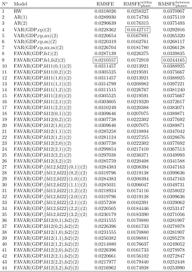
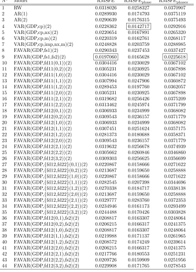
Figure 1 shows seasonally unadjusted as well as seasonally adjusted GDP series. The first five observations get lost to make the seasonally unadjusted series stationary. If the rest part is divided in halves, the first half contains a smooth growth (a matter to calculate within-a-business-cycle-phase RMSFEs), whereas the second half contains a pronounced switch of business cycle phases from growth to a deep recession (a matter to calculate between-business-cycle-phases RMSFEs). Table 1 to Table 5 show root mean squared forecast errors (RMSFE) for the full sample, the first half of the sample (RMSFEwithinphase) and

the second half of the sample (RMSFEbetweenphases ) from pseudo real-time nowcasts

beginning at sample size 19 from a random walk (RW), autoregressive (AR) and vector autoregressive (VAR) models versus static, dynamic and mixed factor-augmented VAR (FAVAR) models, where factors are formed from various com-binations of variables cp, imp, exp, nx and m. In these tables, VAR models are specified by their endogenous variables (first parenthesis) and a lag order (second parenthesis). FAVAR models are specified by their endogenous vari-ables (first parenthesis) and a lag order (second parenthesis). Static factors are specified by a combination of three symbols ‘fsi’, where the first symbol ‘f’ de-notes that the variable is a factor, the second symbol ‘s’ means that the factor is obtained in a static manner, and the third symbol ‘i’ denotes the order of the factor. In this paper, we will use only two kinds of static factors: ‘fs1’ and ‘fs2’, which are static first and second common factors, accordingly. Dynamic factors are specified by a symbol combination ‘fdij(p,q)’, where ‘f’ stands for being a factor, ‘d’ stands for being a dynamic one, ‘ij’ stands for being the i-th out of j simultaneously estimated factors, and the numbers ‘(p,q)’ mean that the factor’s dynamics in (4) are specified by an ARMA(p,q) process. Note that for simplicity, the indiosyncratic component in (4) is set to follow an AR(1) for all dynamic factors, regardless of their ARMA specifications. The least RMSFE for each sample space is framed.

(10)

It is shown that the best nowcasting performance for the within-a-phase period is obtained by a parsimonious VAR, while for the whole series as well as for the between-phases period - by a mixed FAVAR, where the first factor is taken from a dynamic two-factor model with ARMA(1,2), whereas the second factor is the second static common factor. Finally, Table 5 shows the results for the GDP nowcasting performance using four endogenous explanatory variables,cp,

imp, nx, andm. This variable combination is interesting because (logged)nx

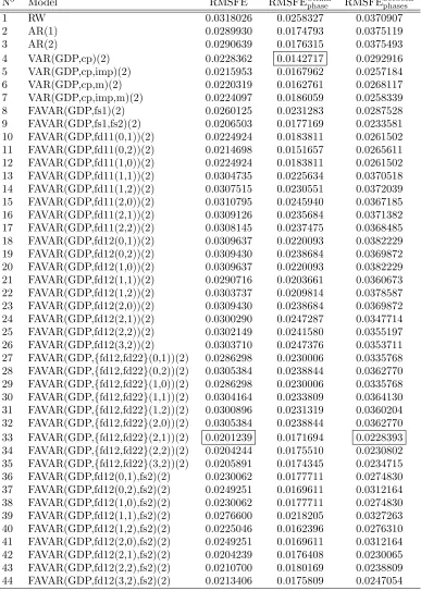
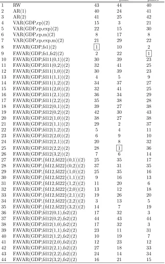
is a difference between (logged)expand impand, thus, might resemble a case if one used a large number of both disaggregated and aggregated variables to form factors, since, in that case, some of the variables might be linear combi-nations of other variables. Thus, Table 5 shows the nowcasting results when the factor-forming variables are not carefully preselected. It is shown that the static two-factor FAVAR performs slightly better in this case compared to when static factors are formed only from a three-variable combination, {cp,nx,m}or

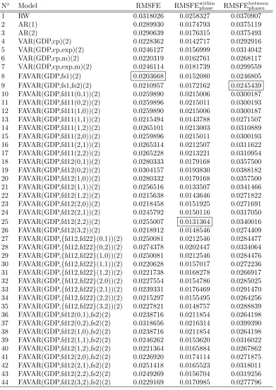
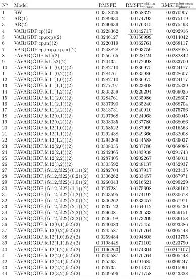
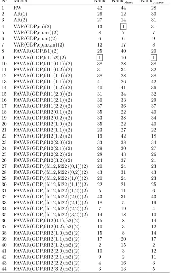
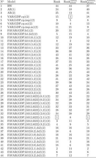
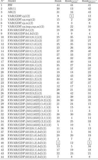
{cp,imp,m} (see Table 1 or Table 2, respectively), giving the best nowcasting performance for the whole series as well as for the between-phases period. On the contrary, the best-performing dynamic factor model using a set of endoge-nous explanatory variables{cp,imp,m}(see Table 2) now performs considerably worse, when addingnxto the set of variables for factor extraction. The latter observation might suggest that the performance of dynamic factors is less ro-bust to a slight change of variables than that of static factors. To examine the issue, Table 6 to Table 10 show the ranking of the models reported in Table 1 to Table 5. The ranking for a static two-factor FAVAR (model 9) for the whole series, within-a-phase, and between-phases period is{1,10,1}for variable set {cp,nx,m}, {5,15,4} for variable set {cp,imp,m}, {2,22,1} for variable set

{cp,exp,m}, {5,9,4} for variable set{cp,imp,exp,m}, and{1,11,1} for variable set {cp,imp,nx,m}, out of overall 44 models. The ranking for a dynamic two-factor FAVAR(2,1) (model 33), the model which performs the best in Table 2, for the whole series, within-a-phase, and between-phases period is{18,5,19}for variable set{cp,nx,m},{1,8,1}for variable set{cp,imp,m},{19,26,20}for vari-able set{cp,exp,m},{10,4,14}for variable set{cp,imp,exp,m}, and{44,44,40}

for variable set {cp,imp,nx,m}, out of overall 44 models. We can see that the ranking of the static FAVAR seems more stable with respect to change of vari-ables than that of the dynamic FAVAR. Indeed, the dynamic factor model turns from the best-performing nowcasting model for the set of variables{cp,imp,m}, to the worst nowcasting model for the set of variables {cp,imp,nx,m}, where the only difference between the variable sets is an addition of a single variable to the former set. To take into account the changes in factor models’ nowcast-ing performance with respect to a slight change of the set of variables, from which factors are extracted, Table 11 shows the models’ ranking based on the mean rank calculated from the rankings reported in Table 6 to Table 10. It is shown that, although some of the mixed FAVAR perform decently, static FAVAR model appears to be the most precise and robust with respect to the change of the factor-forming set of variables for the whole series as well as for the between-phases period. Also, if one considers one-factor models, it is shown that one-factor static FAVAR outperforms one-factor dynamic FAVARs except for the within-a-phase period, where the performance is similar.

(11)

compared to the ranking in Table 11. With minor changes, Table 12 shows the same pattern as Table 11.

Finally, just for illustrative purposes, Figure 3 to Figure 11 show stationary GDP, static first common factor, and dynamic first common factor formed from the variable set {cp,nx,m}, where dynamic factors are generated by various ARMA specifications, starting from ARMA(0,1) and ending at ARMA(2,2). It is shown that, regardless of dynamics specification, dynamic factors fail to detect the timing and depth of the latest recession, the period of which is colored gray in the figures.

4 Conclusions

The choice between static and dynamic factors in now-/forecasting GDP is un-resolved. Some papers find dynamic factors superior over the static ones. Other papers find little or no advantage of dynamic over static factors. On top of them, there are papers that argue for static over dynamic factors. Another debate is going on regarding large-scale versus small-scale factor models. Given the lack of empirical evidence or rationale for large-scale factor models in now-/forecasting GDP, we build a parsimonious, small-scale factor model for the GDP of one of the hardest hit economies during the latest recession to study the exact dynamic versus static factor model performance along a business cycle, with an empha-sis placing on nowcasting performance during a pronounced switch of business cycle phases due to the latest recession. We compare the factor models’ now-casting performance to a random walk, autoregressive and the best-performing nowcasting models at our hands, which are VAR models. It is shown that a small-scale static FAVAR model tends to improve upon the nowcasting perfor-mance of the VAR models during the switch business cycle phases (between business cycle phases), while exact dynamic factor models tend to fail to detect the timing and depth of the recession regardless of ARMA specifications. As regards the period of smooth economic growth (within a business cycle phase), static and dynamic factor models appear to show similar performance with po-tentially slight superiority of dynamic factor models if the factor-forming set of variables and factor dynamics are carefully selected.

References

[1] Ajevskis, V. and G. Davidsons (2008), “Dynamic factor models in forecast-ing Latvia’s gross domestic product”, Workforecast-ing papers 2008/02, Latvijas Banka

[2] Banerjee, A., M. Marcellino and I. Masten (2010), “Forecasting with factor-augmented error correction models”, Discussion Papers 09-06R, Depart-ment of Economics, University of Birmingham

[3] Boivin, J. and S. Ng (2003), “Are mode data always better for factor analy-sis?”, NBER Working Papers 9829, National Bureau of Economic Research, Inc.

(12)

[5] Camacho, M., G. Perez-Quiros and P. Poncela (2010), “Markov-switching dynamic factor models in real time”, forthcoming

[6] Chauvet, M. (1998), “An econometric characterization of business cycle dy-namics with factor structure and regime switches”,International Economic Review, 39(4), 969-96

[7] Chauvet, M. and J. Hamilton (2005), “Dating business cycle turning points”, NBER Working Papers 11422

[8] D’Agostino, A. and D. Giannone (2007), “Comparing alternative predic-tors based on large-panel factor models”, CEPR Discussion Papers 6564, C.E.P.R. Discussion Papers

[9] Doz, C. and F. Lenglart (1999), “Analyse factorielle dynamique: test du nombre de facteurs, estimation et application à l’enquête de conjoncture dans l’industrie”,Annales d’ Économie et de Statistique, No. 54, 91-127

[10] Dubois, E. and Michaux, E. (2010), “Grocer 1.41: an econometric toolbox for Scilab”, available at http://dubois.ensae.net/grocer.html

[11] Gupta, R. and A. Kabundi (2008), “Forecasting macroeconomic variables using large datasets: dynamic factor models versus large-scale BVARs”, Working Papers 200816, University of Pretoria, Department of Economics

[12] Gupta, R. and A. Kabundi (2009), “A large factor model for forecasting macroeconomic variables in South Africa”, Working Papers 137, Economic Research Southern Africa, University of Cape Town

[13] Kim, M. J. and J. S. Yoo (1995),“New index of coincident indicators: A multivariate Markov switching factor model approach”,Journal of Mone-tary Economics, 36(3), 607-630

[14] Kim, C. J. and C. R. Nelson (1998), “Business cycle turning points, a new coincident index, and tests of duration dependence based on a dynamic factor model with regime switching”,Review of Economics and Statistics, 80(2), 188-201

[15] Marcellino, M. and C. Schumacher (2008), “Factor-MIDAS for now- and forecasting with ragged-edge data: A model comparison for German GDP”, CEPR Discussion Papers 6708

[16] Reijer, A. H. J. den (2005), “Forecasting Dutch GDP using large scale factor models”, DNB Working Papers 028, Netherlands Central Bank, Research Department

[17] Schneider, M. and M. Spitzer (2004), “Forecasting Austrian GDP using the generalized dynamic factor model”, Working Papers 89, Oesterreichische Nationalbank (Austrian Central Bank)

(13)

[19] Siliverstovs, B., and K. A. Kholodilin (2010), “Assessing the real-time in-formational content of macroeconomic data releases for now-/forecasting GDP: evidence for Switzerland”, KOF Working papers 10-251, KOF Swiss Economic Institute, ETH Zurich

[20] Stock, J. H. and M. Watson (1998), “Diffusion indexes”, NBER Working Paper, No. 6702

(14)

[image:14.612.149.445.142.314.2]

Appendix

(15)

No _Model _RMSFE _RMSFEwithin

phase RMSFEbetweenphases

1 RW 0.0318026 0.0258327 0.0370907

2 AR(1) 0.0289930 0.0174793 0.0375119

3 AR(2) 0.0290639 0.0176315 0.0375493

4 VAR(GDP,cp)(2) 0.0228362 0.0142717 0.0292916

[image:15.612.127.514.74.622.2]

5 VAR(GDP,cp,nx)(2) 0.0220654 0.0167891 0.0265320 6 VAR(GDP,cp,m)(2) 0.0220319 0.0162761 0.0268117 7 VAR(GDP,cp,nx,m)(2) 0.0226704 0.0181780 0.0266128 8 FAVAR(GDP,fs1)(2) 0.0287139 0.0226375 0.0339835 9 FAVAR(GDP,fs1,fs2)(2) 0.0210557 0.0172919 0.0244165 10 FAVAR(GDP,fd11(0,1))(2) 0.0311457 0.0213921 0.0388925 11 FAVAR(GDP,fd11(0,2))(2) 0.0305525 0.0219591 0.0375667 12 FAVAR(GDP,fd11(1,0))(2) 0.0311457 0.0213921 0.0388925 13 FAVAR(GDP,fd11(1,1))(2) 0.0314799 0.0208982 0.0397221 14 FAVAR(GDP,fd11(1,2))(2) 0.0311515 0.0226767 0.0381240 15 FAVAR(GDP,fd11(2,0))(2) 0.0305525 0.0219591 0.0375667 16 FAVAR(GDP,fd11(2,1))(2) 0.0303605 0.0219320 0.0372617 17 FAVAR(GDP,fd11(2,2))(2) 0.0310249 0.0220388 0.0383071 18 FAVAR(GDP,fd12(0,1))(2) 0.0309646 0.0207075 0.0389871 19 FAVAR(GDP,fd12(0,2))(2) 0.0307738 0.0222302 0.0377692 20 FAVAR(GDP,fd12(1,0))(2) 0.0309646 0.0207075 0.0389871 21 FAVAR(GDP,fd12(1,1))(2) 0.0285258 0.0210894 0.0347042 22 FAVAR(GDP,fd12(1,2))(2) 0.0281124 0.0227255 0.0328676 23 FAVAR(GDP,fd12(2,0))(2) 0.0307738 0.0222302 0.0377692 24 FAVAR(GDP,fd12(2,1))(2) 0.0299854 0.0217410 0.0367513 25 FAVAR(GDP,fd12(2,2))(2) 0.0297038 0.0236371 0.0349993 26 FAVAR(GDP,fd12(3,2))(2) 0.0285759 0.0220408 0.0341588 27 FAVAR(GDP,{fd12,fd22}(0,1))(2) 0.0284383 0.0208394 0.0347163 28 FAVAR(GDP,{fd12,fd22}(0,2))(2) 0.0319796 0.0219138 0.0399636 29 FAVAR(GDP,{fd12,fd22}(1,0))(2) 0.0284383 0.0208394 0.0347163 30 FAVAR(GDP,{fd12,fd22}(1,1))(2) 0.0285031 0.0206047 0.0349731 31 FAVAR(GDP,{fd12,fd22}(1,2))(2) 0.0218924 0.0174116 0.0258022 32 FAVAR(GDP,{fd12,fd22}(2,0))(2) 0.0319796 0.0219138 0.0399636 33 FAVAR(GDP,{fd12,fd22}(2,1))(2) 0.0257208 0.0162391 0.0329062 34 FAVAR(GDP,{fd12,fd22}(2,2))(2) 0.0220505 0.0184446 0.0253147 35 FAVAR(GDP,{fd12,fd22}(3,2))(2) 0.0230179 0.0183390 0.0271056 36 FAVAR(GDP,fd12(0,1),fs2)(2) 0.0231555 0.0170880 0.0281907 37 FAVAR(GDP,fd12(0,2),fs2)(2) 0.0226396 0.0161733 0.0278978 38 FAVAR(GDP,fd12(1,0),fs2)(2) 0.0231555 0.0170880 0.0281907 39 FAVAR(GDP,fd12(1,1),fs2)(2) 0.0250382 0.0198881 0.0295278 40 FAVAR(GDP,fd12(1,2),fs2)(2) 0.0214880 0.0176637 0.0249052 41 FAVAR(GDP,fd12(2,0),fs2)(2) 0.0226396 0.0161733 0.0278978 42 FAVAR(GDP,fd12(2,1),fs2)(2) 0.0220661 0.0156102 0.0272847 43 FAVAR(GDP,fd12(2,2),fs2)(2) 0.0217977 0.0179440 0.0252448 44 FAVAR(GDP,fd12(3,2),fs2)(2) 0.0216962 0.0174938 0.0253990

Table 1: A comparison of pseudo real-time nowcasting performance from RW, AR, VAR, static, dynamic and mixed FAVAR models in terms of RMSFE for the full sample, first half of the sample (RMSFEwithinphase) and second half of the

sample (RMSFEbetweenphases ). Factors are formed from cp, nx and m. The least

(16)

1 RW 0.0318026 0.0258327 0.0370907

2 AR(1) 0.0289930 0.0174793 0.0375119

3 AR(2) 0.0290639 0.0176315 0.0375493

4 VAR(GDP,cp)(2) 0.0228362 0.0142717 0.0292916

[image:16.612.129.516.80.623.2]

5 VAR(GDP,cp,imp)(2) 0.0215953 0.0167962 0.0257184 6 VAR(GDP,cp,m)(2) 0.0220319 0.0162761 0.0268117 7 VAR(GDP,cp,imp,m)(2) 0.0224097 0.0186059 0.0258339 8 FAVAR(GDP,fs1)(2) 0.0260125 0.0231283 0.0287528 9 FAVAR(GDP,fs1,fs2)(2) 0.0206503 0.0177169 0.0233581 10 FAVAR(GDP,fd11(0,1))(2) 0.0224924 0.0183811 0.0261502 11 FAVAR(GDP,fd11(0,2))(2) 0.0214698 0.0151657 0.0265611 12 FAVAR(GDP,fd11(1,0))(2) 0.0224924 0.0183811 0.0261502 13 FAVAR(GDP,fd11(1,1))(2) 0.0304735 0.0225634 0.0370518 14 FAVAR(GDP,fd11(1,2))(2) 0.0307515 0.0230551 0.0372039 15 FAVAR(GDP,fd11(2,0))(2) 0.0310795 0.0245940 0.0367185 16 FAVAR(GDP,fd11(2,1))(2) 0.0309126 0.0235684 0.0371382 17 FAVAR(GDP,fd11(2,2))(2) 0.0308145 0.0237475 0.0368485 18 FAVAR(GDP,fd12(0,1))(2) 0.0309637 0.0220093 0.0382229 19 FAVAR(GDP,fd12(0,2))(2) 0.0309430 0.0238684 0.0369872 20 FAVAR(GDP,fd12(1,0))(2) 0.0309637 0.0220093 0.0382229 21 FAVAR(GDP,fd12(1,1))(2) 0.0290716 0.0203661 0.0360673 22 FAVAR(GDP,fd12(1,2))(2) 0.0303737 0.0209814 0.0378587 23 FAVAR(GDP,fd12(2,0))(2) 0.0309430 0.0238684 0.0369872 24 FAVAR(GDP,fd12(2,1))(2) 0.0300290 0.0247287 0.0347714 25 FAVAR(GDP,fd12(2,2))(2) 0.0302149 0.0241580 0.0355197 26 FAVAR(GDP,fd12(3,2))(2) 0.0303710 0.0247376 0.0353711 27 FAVAR(GDP,{fd12,fd22}(0,1))(2) 0.0286298 0.0230006 0.0335768 28 FAVAR(GDP,{fd12,fd22}(0,2))(2) 0.0305384 0.0238844 0.0362770 29 FAVAR(GDP,{fd12,fd22}(1,0))(2) 0.0286298 0.0230006 0.0335768 30 FAVAR(GDP,{fd12,fd22}(1,1))(2) 0.0304164 0.0233809 0.0364130 31 FAVAR(GDP,{fd12,fd22}(1,2))(2) 0.0300896 0.0231319 0.0360204 32 FAVAR(GDP,{fd12,fd22}(2,0))(2) 0.0305384 0.0238844 0.0362770 33 FAVAR(GDP,{fd12,fd22}(2,1))(2) 0.0201239 0.0171694 0.0228393 34 FAVAR(GDP,{fd12,fd22}(2,2))(2) 0.0204244 0.0175510 0.0230802 35 FAVAR(GDP,{fd12,fd22}(3,2))(2) 0.0205891 0.0174345 0.0234715 36 FAVAR(GDP,fd12(0,1),fs2)(2) 0.0230062 0.0177711 0.0274830 37 FAVAR(GDP,fd12(0,2),fs2)(2) 0.0249251 0.0169611 0.0312164 38 FAVAR(GDP,fd12(1,0),fs2)(2) 0.0230062 0.0177711 0.0274830 39 FAVAR(GDP,fd12(1,1),fs2)(2) 0.0276600 0.0218205 0.0327263 40 FAVAR(GDP,fd12(1,2),fs2)(2) 0.0225046 0.0162396 0.0276310 41 FAVAR(GDP,fd12(2,0),fs2)(2) 0.0249251 0.0169611 0.0312164 42 FAVAR(GDP,fd12(2,1),fs2)(2) 0.0204239 0.0176408 0.0230065 43 FAVAR(GDP,fd12(2,2),fs2)(2) 0.0210700 0.0180169 0.0238809 44 FAVAR(GDP,fd12(3,2),fs2)(2) 0.0213406 0.0175809 0.0247054

sample (RMSFEbetweenphases ). Factors are formed fromcp, imp and m. The least

(17)

1 RW 0.0318026 0.0258327 0.0370907

2 AR(1) 0.0289930 0.0174793 0.0375119

3 AR(2) 0.0290639 0.0176315 0.0375493

4 VAR(GDP,cp)(2) 0.0228362 0.0142717 0.0292916

[image:17.612.129.520.74.626.2]

5 VAR(GDP,cp,exp)(2) 0.0246127 0.0156999 0.0314042 6 VAR(GDP,cp,m)(2) 0.0220319 0.0162761 0.0268117 7 VAR(GDP,cp,exp,m)(2) 0.0246114 0.0181739 0.0299559 8 FAVAR(GDP,fs1)(2) 0.0203668 0.0152080 0.0246805 9 FAVAR(GDP,fs1,fs2)(2) 0.0210957 0.0172162 0.0245439 10 FAVAR(GDP,fd11(0,1))(2) 0.0259890 0.0215006 0.0300187 11 FAVAR(GDP,fd11(0,2))(2) 0.0259896 0.0215011 0.0300193 12 FAVAR(GDP,fd11(1,0))(2) 0.0259890 0.0215006 0.0300187 13 FAVAR(GDP,fd11(1,1))(2) 0.0215494 0.0143788 0.0271507 14 FAVAR(GDP,fd11(1,2))(2) 0.0265101 0.0213003 0.0310889 15 FAVAR(GDP,fd11(2,0))(2) 0.0259896 0.0215011 0.0300193 16 FAVAR(GDP,fd11(2,1))(2) 0.0265314 0.0212507 0.0311622 17 FAVAR(GDP,fd11(2,2))(2) 0.0265228 0.0213221 0.0310954 18 FAVAR(GDP,fd12(0,1))(2) 0.0280333 0.0179168 0.0357500 19 FAVAR(GDP,fd12(0,2))(2) 0.0304157 0.0193830 0.0388182 20 FAVAR(GDP,fd12(1,0))(2) 0.0280332 0.0179168 0.0357500 21 FAVAR(GDP,fd12(1,1))(2) 0.0256516 0.0133507 0.0341466 22 FAVAR(GDP,fd12(1,2))(2) 0.0215638 0.0143646 0.0271822 23 FAVAR(GDP,fd12(2,0))(2) 0.0218458 0.0151925 0.0271691 24 FAVAR(GDP,fd12(2,1))(2) 0.0245792 0.0150116 0.0317050 25 FAVAR(GDP,fd12(2,2))(2) 0.0255007 0.0131364 0.0340016 26 FAVAR(GDP,fd12(3,2))(2) 0.0218912 0.0148546 0.0274409 27 FAVAR(GDP,{fd12,fd22}(0,1))(2) 0.0250081 0.0212546 0.0284477 28 FAVAR(GDP,{fd12,fd22}(0,2))(2) 0.0274378 0.0202447 0.0334064 29 FAVAR(GDP,{fd12,fd22}(1,0))(2) 0.0250081 0.0212546 0.0284476 30 FAVAR(GDP,{fd12,fd22}(1,1))(2) 0.0220628 0.0157017 0.0272236 31 FAVAR(GDP,{fd12,fd22}(1,2))(2) 0.0221738 0.0168278 0.0266917 32 FAVAR(GDP,{fd12,fd22}(2,0))(2) 0.0227554 0.0154786 0.0285025 33 FAVAR(GDP,{fd12,fd22}(2,1))(2) 0.0239331 0.0176469 0.0291470 34 FAVAR(GDP,{fd12,fd22}(2,2))(2) 0.0215297 0.0155495 0.0264256 35 FAVAR(GDP,{fd12,fd22}(3,2))(2) 0.0227821 0.0148757 0.0288839 36 FAVAR(GDP,fd12(0,1),fs2)(2) 0.0238716 0.0211854 0.0264198 37 FAVAR(GDP,fd12(0,2),fs2)(2) 0.0318656 0.0216314 0.0399390 38 FAVAR(GDP,fd12(1,0),fs2)(2) 0.0238716 0.0211854 0.0264198 39 FAVAR(GDP,fd12(1,1),fs2)(2) 0.0246262 0.0153620 0.0316022 40 FAVAR(GDP,fd12(1,2),fs2)(2) 0.0221364 0.0165884 0.0267862 41 FAVAR(GDP,fd12(2,0),fs2)(2) 0.0226920 0.0174114 0.0271875 42 FAVAR(GDP,fd12(2,1),fs2)(2) 0.0251418 0.0165523 0.0318011 43 FAVAR(GDP,fd12(2,2),fs2)(2) 0.0249269 0.0156704 0.0319256 44 FAVAR(GDP,fd12(3,2),fs2)(2) 0.0229169 0.0170985 0.0277796

(18)

1 RW 0.0318026 0.0258327 0.0370907

2 AR(1) 0.0289930 0.0174793 0.0375119

3 AR(2) 0.0290639 0.0176315 0.0375493

4 VAR(GDP,cp)(2) 0.0228362 0.0142717 0.0292916

[image:18.612.127.515.72.626.2]

5 VAR(GDP,cp,exp)(2) 0.0246127 0.0156999 0.0314042 6 VAR(GDP,cp,m)(2) 0.0220319 0.0162761 0.0268117 7 VAR(GDP,cp,imp,exp,m)(2) 0.0248828 0.0203759 0.0288985 8 FAVAR(GDP,fs1)(2) 0.0256165 0.0228124 0.0282842 9 FAVAR(GDP,fs1,fs2)(2) 0.0204351 0.0172098 0.0233700 10 FAVAR(GDP,fd11(0,1))(2) 0.0282710 0.0236975 0.0324177 11 FAVAR(GDP,fd11(0,2))(2) 0.0284761 0.0235986 0.0328607 12 FAVAR(GDP,fd11(1,0))(2) 0.0282710 0.0236975 0.0324177 13 FAVAR(GDP,fd11(1,1))(2) 0.0277797 0.0223808 0.0325339 14 FAVAR(GDP,fd11(1,2))(2) 0.0305259 0.0229294 0.0369025 15 FAVAR(GDP,fd11(2,0))(2) 0.0284761 0.0235986 0.0328607 16 FAVAR(GDP,fd11(2,1))(2) 0.0307390 0.0235240 0.0368704 17 FAVAR(GDP,fd11(2,2))(2) 0.0313731 0.0240910 0.0375756 18 FAVAR(GDP,fd12(0,1))(2) 0.0297968 0.0224068 0.0360045 19 FAVAR(GDP,fd12(0,2))(2) 0.0308035 0.0237780 0.0368086 20 FAVAR(GDP,fd12(1,0))(2) 0.0258522 0.0187909 0.0316563 21 FAVAR(GDP,fd12(1,1))(2) 0.0292438 0.0249366 0.0332008 22 FAVAR(GDP,fd12(1,2))(2) 0.0294269 0.0244588 0.0339027 23 FAVAR(GDP,fd12(2,0))(2) 0.0308035 0.0237780 0.0368086 24 FAVAR(GDP,fd12(2,1))(2) 0.0242365 0.0183938 0.0291743 25 FAVAR(GDP,fd12(2,2))(2) 0.0287405 0.0202267 0.0356011 26 FAVAR(GDP,fd12(3,2))(2) 0.0303592 0.0248137 0.0352937 27 FAVAR(GDP,{fd12,fd22}(0,1))(2) 0.0282704 0.0237917 0.0323435 28 FAVAR(GDP,{fd12,fd22}(0,2))(2) 0.0306262 0.0233457 0.0367971 29 FAVAR(GDP,{fd12,fd22}(1,0))(2) 0.0260043 0.0216621 0.0299229 30 FAVAR(GDP,{fd12,fd22}(1,1))(2) 0.0207281 0.0175698 0.0236162 31 FAVAR(GDP,{fd12,fd22}(1,2))(2) 0.0203595 0.0174192 0.0230678 32 FAVAR(GDP,{fd12,fd22}(2,0))(2) 0.0306262 0.0233457 0.0367971 33 FAVAR(GDP,{fd12,fd22}(2,1))(2) 0.0237122 0.0164012 0.0295430 34 FAVAR(GDP,{fd12,fd22}(2,2))(2) 0.0296081 0.0220533 0.0359151 35 FAVAR(GDP,{fd12,fd22}(3,2))(2) 0.0206198 0.0173209 0.0236158 36 FAVAR(GDP,fd12(0,1),fs2)(2) 0.0240083 0.0175455 0.0293386 37 FAVAR(GDP,fd12(0,2),fs2)(2) 0.0245587 0.0170764 0.0305448 38 FAVAR(GDP,fd12(1,0),fs2)(2) 0.0259484 0.0194808 0.0313755 39 FAVAR(GDP,fd12(1,1),fs2)(2) 0.0198448 0.0171102 0.0223790 40 FAVAR(GDP,fd12(1,2),fs2)(2) 0.0196263 0.0174304 0.0217107 41 FAVAR(GDP,fd12(2,0),fs2)(2) 0.0245587 0.0170764 0.0305448 42 FAVAR(GDP,fd12(2,1),fs2)(2) 0.0255631 0.0191685 0.0309247 43 FAVAR(GDP,fd12(2,2),fs2)(2) 0.0267351 0.0211375 0.0315991 44 FAVAR(GDP,fd12(3,2),fs2)(2) 0.0209596 0.0171758 0.0243328

sample (RMSFEbetweenphases ). Factors are formed fromcp, imp, exp and m. The

(19)

1 RW 0.0318026 0.0258327 0.0370907

2 AR(1) 0.0289930 0.0174793 0.0375119

3 AR(2) 0.0290639 0.0176315 0.0375493

4 VAR(GDP,cp)(2) 0.0228362 0.0142717 0.0292916

[image:19.612.127.520.81.626.2]

5 VAR(GDP,cp,nx)(2) 0.0220654 0.0167891 0.0265320 6 VAR(GDP,cp,m)(2) 0.0220319 0.0162761 0.0268117 7 VAR(GDP,cp,imp,nx,m)(2) 0.0248828 0.0203759 0.0288985 8 FAVAR(GDP,fs1)(2) 0.0290343 0.0237453 0.0337427 9 FAVAR(GDP,fs1,fs2)(2) 0.0197060 0.0165628 0.0225618 10 FAVAR(GDP,fd11(0,1))(2) 0.0304416 0.0230029 0.0367102 11 FAVAR(GDP,fd11(0,2))(2) 0.0305231 0.0230925 0.0367898 12 FAVAR(GDP,fd11(1,0))(2) 0.0304416 0.0230029 0.0367102 13 FAVAR(GDP,fd11(1,1))(2) 0.0307994 0.0247906 0.0360872 14 FAVAR(GDP,fd11(1,2))(2) 0.0289453 0.0197760 0.0362057 15 FAVAR(GDP,fd11(2,0))(2) 0.0305231 0.0230925 0.0367898 16 FAVAR(GDP,fd11(2,1))(2) 0.0319682 0.0256426 0.0375209 17 FAVAR(GDP,fd11(2,2))(2) 0.0313462 0.0245974 0.0371799 18 FAVAR(GDP,fd12(0,1))(2) 0.0306933 0.0234999 0.0368082 19 FAVAR(GDP,fd12(0,2))(2) 0.0309543 0.0236157 0.0371779 20 FAVAR(GDP,fd12(1,0))(2) 0.0306933 0.0234999 0.0368082 21 FAVAR(GDP,fd12(1,1))(2) 0.0307451 0.0251624 0.0357175 22 FAVAR(GDP,fd12(1,2))(2) 0.0281373 0.0180688 0.0358371 23 FAVAR(GDP,fd12(2,0))(2) 0.0309543 0.0236157 0.0371779 24 FAVAR(GDP,fd12(2,1))(2) 0.0319632 0.0256678 0.0374939 25 FAVAR(GDP,fd12(2,2))(2) 0.0305662 0.0260846 0.0346860 26 FAVAR(GDP,fd12(3,2))(2) 0.0309303 0.0256625 0.0356699 27 FAVAR(GDP,{fd12,fd22}(0,1))(2) 0.0220867 0.0158666 0.0271622 28 FAVAR(GDP,{fd12,fd22}(0,2))(2) 0.0213687 0.0159650 0.0258888 29 FAVAR(GDP,{fd12,fd22}(1,0))(2) 0.0220867 0.0158666 0.0271622 30 FAVAR(GDP,{fd12,fd22}(1,1))(2) 0.0282545 0.0207398 0.0344696 31 FAVAR(GDP,{fd12,fd22}(1,2))(2) 0.0270338 0.0184717 0.0338138 32 FAVAR(GDP,{fd12,fd22}(2,0))(2) 0.0213687 0.0159650 0.0258888 33 FAVAR(GDP,{fd12,fd22}(2,1))(2) 0.0329777 0.0283760 0.0372353 34 FAVAR(GDP,{fd12,fd22}(2,2))(2) 0.0234946 0.0161173 0.0293499 35 FAVAR(GDP,{fd12,fd22}(3,2))(2) 0.0244488 0.0170426 0.0303828 36 FAVAR(GDP,fd12(0,1),fs2)(2) 0.0208817 0.0163307 0.0248064 37 FAVAR(GDP,fd12(0,2),fs2)(2) 0.0206215 0.0166317 0.0241375 38 FAVAR(GDP,fd12(1,0),fs2)(2) 0.0208817 0.0163307 0.0248064 39 FAVAR(GDP,fd12(1,1),fs2)(2) 0.0219988 0.0171137 0.0261965 40 FAVAR(GDP,fd12(1,2),fs2)(2) 0.0208572 0.0174249 0.0239614 41 FAVAR(GDP,fd12(2,0),fs2)(2) 0.0206215 0.0166317 0.0241375 42 FAVAR(GDP,fd12(2,1),fs2)(2) 0.0217766 0.0180553 0.0251231 43 FAVAR(GDP,fd12(2,2),fs2)(2) 0.0209726 0.0159909 0.0251956 44 FAVAR(GDP,fd12(3,2),fs2)(2) 0.0229908 0.0171765 0.0278543

sample (RMSFEbetweenphases ). Factors are formed fromcp,imp,nxandm. The least

(20)

No _Model _Rank _Rankwithin

phase Rankbetweenphases

1 RW 42 44 28

2 AR(1) 26 12 30

3 AR(2) 27 14 31

4 VAR(GDP,cp)(2) 13 1 31

5 VAR(GDP,cp,nx)(2) 8 7 7

6 VAR(GDP,cp,m)(2) 6 6 9

7 VAR(GDP,cp,nx,m)(2) 12 17 8

8 FAVAR(GDP,fs1)(2) 25 40 20

9 FAVAR(GDP,fs1,fs2)(2) 1 10 1

10 FAVAR(GDP,fd11(0,1))(2) 38 28 38

11 FAVAR(GDP,fd11(0,2))(2) 31 34 32

12 FAVAR(GDP,fd11(1,0))(2) 38 28 38

13 FAVAR(GDP,fd11(1,1))(2) 41 26 42

14 FAVAR(GDP,fd11(1,2))(2) 40 41 36

15 FAVAR(GDP,fd11(2,0))(2) 31 34 32

16 FAVAR(GDP,fd11(2,1))(2) 30 33 29

17 FAVAR(GDP,fd11(2,2))(2) 37 36 37

18 FAVAR(GDP,fd12(0,1))(2) 35 22 40

19 FAVAR(GDP,fd12(0,2))(2) 33 38 34

20 FAVAR(GDP,fd12(1,0))(2) 35 22 40

21 FAVAR(GDP,fd12(1,1))(2) 23 27 22

22 FAVAR(GDP,fd12(1,2))(2) 19 42 18

23 FAVAR(GDP,fd12(2,0))(2) 33 38 34

24 FAVAR(GDP,fd12(2,1))(2) 29 30 27

25 FAVAR(GDP,fd12(2,2))(2) 28 43 26

26 FAVAR(GDP,fd12(3,2))(2) 24 37 21

27 FAVAR(GDP,{fd12,fd22}(0,1))(2) 20 24 23 28 FAVAR(GDP,{fd12,fd22}(0,2))(2) 43 31 43 29 FAVAR(GDP,{fd12,fd22}(1,0))(2) 20 24 23 30 FAVAR(GDP,{fd12,fd22}(1,1))(2) 22 21 25 31 FAVAR(GDP,{fd12,fd22}(1,2))(2) 5 11 6 32 FAVAR(GDP,{fd12,fd22}(2,0))(2) 43 31 43 33 FAVAR(GDP,{fd12,fd22}(2,1))(2) 18 5 19 34 FAVAR(GDP,{fd12,fd22}(2,2))(2) 7 19 4 35 FAVAR(GDP,{fd12,fd22}(3,2))(2) 14 18 10

36 FAVAR(GDP,fd12(0,1),fs2)(2) 15 8 14

37 FAVAR(GDP,fd12(0,2),fs2)(2) 10 3 12

38 FAVAR(GDP,fd12(1,0),fs2)(2) 15 8 14

39 FAVAR(GDP,fd12(1,1),fs2)(2) 17 20 17

40 FAVAR(GDP,fd12(1,2),fs2)(2) 2 15 2

41 FAVAR(GDP,fd12(2,0),fs2)(2) 10 3 12

42 FAVAR(GDP,fd12(2,1),fs2)(2) 9 2 11

43 FAVAR(GDP,fd12(2,2),fs2)(2) 4 16 3

[image:20.612.130.469.91.635.2]

44 FAVAR(GDP,fd12(3,2),fs2)(2) 3 13 5

(21)

1 RW 44 44 37

2 AR(1) 24 10 40

3 AR(2) 25 13 41

4 VAR(GDP,cp)(2) 15 1 18

5 VAR(GDP,cp,imp)(2) 9 5 8

6 VAR(GDP,cp,m)(2) 10 4 13

7 VAR(GDP,cp,imp,m)(2) 11 21 9

8 FAVAR(GDP,fs1)(2) 20 31 17

10 FAVAR(GDP,fd11(0,1))(2) 12 19 10

11 FAVAR(GDP,fd11(0,2))(2) 8 2 12

12 FAVAR(GDP,fd11(1,0))(2) 12 19 10

13 FAVAR(GDP,fd11(1,1))(2) 33 27 36

14 FAVAR(GDP,fd11(1,2))(2) 36 30 39

15 FAVAR(GDP,fd11(2,0))(2) 43 41 32

16 FAVAR(GDP,fd11(2,1))(2) 38 34 38

17 FAVAR(GDP,fd11(2,2))(2) 37 35 33

18 FAVAR(GDP,fd12(0,1))(2) 41 25 43

19 FAVAR(GDP,fd12(0,2))(2) 39 36 34

20 FAVAR(GDP,fd12(1,0))(2) 41 25 43

21 FAVAR(GDP,fd12(1,1))(2) 26 22 28

22 FAVAR(GDP,fd12(1,2))(2) 31 23 42

23 FAVAR(GDP,fd12(2,0))(2) 39 36 34

24 FAVAR(GDP,fd12(2,1))(2) 27 42 24

25 FAVAR(GDP,fd12(2,2))(2) 29 40 26

26 FAVAR(GDP,fd12(3,2))(2) 30 43 25

27 FAVAR(GDP,{fd12,fd22}(0,1))(2) 22 28 22 28 FAVAR(GDP,{fd12,fd22}(0,2))(2) 34 38 29 29 FAVAR(GDP,{fd12,fd22}(1,0))(2) 22 28 22 30 FAVAR(GDP,{fd12,fd22}(1,1))(2) 32 33 31 31 FAVAR(GDP,{fd12,fd22}(1,2))(2) 28 32 27 32 FAVAR(GDP,{fd12,fd22}(2,0))(2) 34 38 29 33 FAVAR(GDP,{fd12,fd22}(2,1))(2) 1 8 1 34 FAVAR(GDP,{fd12,fd22}(2,2))(2) 3 11 3 35 FAVAR(GDP,{fd12,fd22}(3,2))(2) 4 9 5 36 FAVAR(GDP,fd12(0,1),fs2)(2) 16 16 14

37 FAVAR(GDP,fd12(0,2),fs2)(2) 18 6 19

38 FAVAR(GDP,fd12(1,0),fs2)(2) 16 16 14 39 FAVAR(GDP,fd12(1,1),fs2)(2) 21 24 21

40 FAVAR(GDP,fd12(1,2),fs2)(2) 14 3 16

41 FAVAR(GDP,fd12(2,0),fs2)(2) 18 6 19

42 FAVAR(GDP,fd12(2,1),fs2)(2) 2 14 2

43 FAVAR(GDP,fd12(2,2),fs2)(2) 6 18 6

[image:21.612.131.463.86.632.2]

44 FAVAR(GDP,fd12(3,2),fs2)(2) 7 12 7

(22)

1 RW 43 44 40

2 AR(1) 40 24 41

3 AR(2) 41 25 42

4 VAR(GDP,cp)(2) 15 3 21

5 VAR(GDP,cp,exp)(2) 22 15 30

6 VAR(GDP,cp,m)(2) 8 17 8

7 VAR(GDP,cp,exp,m)(2) 21 29 22

8 FAVAR(GDP,fs1)(2) 1 10 2

10 FAVAR(GDP,fd11(0,1))(2) 30 39 23

11 FAVAR(GDP,fd11(0,2))(2) 32 41 25

12 FAVAR(GDP,fd11(1,0))(2) 30 39 23

13 FAVAR(GDP,fd11(1,1))(2) 4 5 9

14 FAVAR(GDP,fd11(1,2))(2) 34 37 27

15 FAVAR(GDP,fd11(2,0))(2) 32 41 25

16 FAVAR(GDP,fd11(2,1))(2) 36 34 29

17 FAVAR(GDP,fd11(2,2))(2) 35 38 28

18 FAVAR(GDP,fd12(0,1))(2) 39 27 38

19 FAVAR(GDP,fd12(0,2))(2) 42 30 43

20 FAVAR(GDP,fd12(1,0))(2) 38 27 38

21 FAVAR(GDP,fd12(1,1))(2) 29 2 37

22 FAVAR(GDP,fd12(1,2))(2) 5 4 11

23 FAVAR(GDP,fd12(2,0))(2) 6 9 10

24 FAVAR(GDP,fd12(2,1))(2) 20 8 32

25 FAVAR(GDP,fd12(2,2))(2) 28 1 36

26 FAVAR(GDP,fd12(3,2))(2) 7 6 14

36 FAVAR(GDP,fd12(0,1),fs2)(2) 17 32 3

37 FAVAR(GDP,fd12(0,2),fs2)(2) 44 43 44

38 FAVAR(GDP,fd12(1,0),fs2)(2) 17 32 3

39 FAVAR(GDP,fd12(1,1),fs2)(2) 23 11 31

40 FAVAR(GDP,fd12(1,2),fs2)(2) 10 19 7

[image:22.612.130.468.95.633.2]

41 FAVAR(GDP,fd12(2,0),fs2)(2) 12 23 12 42 FAVAR(GDP,fd12(2,1),fs2)(2) 27 18 33 43 FAVAR(GDP,fd12(2,2),fs2)(2) 24 14 34 44 FAVAR(GDP,fd12(3,2),fs2)(2) 16 21 15

(23)

1 RW 44 44 41

2 AR(1) 30 13 42

3 AR(2) 31 16 43

4 VAR(GDP,cp)(2) 9 1 12

5 VAR(GDP,cp,exp)(2) 15 2 20

6 VAR(GDP,cp,m)(2) 8 3 8

7 VAR(GDP,cp,imp,exp,m)(2) 16 22 10

8 FAVAR(GDP,fs1)(2) 18 28 9

10 FAVAR(GDP,fd11(0,1))(2) 25 35 24

11 FAVAR(GDP,fd11(0,2))(2) 27 33 27

12 FAVAR(GDP,fd11(1,0))(2) 25 35 24

13 FAVAR(GDP,fd11(1,1))(2) 23 26 26

14 FAVAR(GDP,fd11(1,2))(2) 37 29 40

15 FAVAR(GDP,fd11(2,0))(2) 27 33 27

16 FAVAR(GDP,fd11(2,1))(2) 40 32 39

17 FAVAR(GDP,fd11(2,2))(2) 43 40 44

18 FAVAR(GDP,fd12(0,1))(2) 35 27 34

19 FAVAR(GDP,fd12(0,2))(2) 41 37 37

20 FAVAR(GDP,fd12(1,0))(2) 19 18 22

21 FAVAR(GDP,fd12(1,1))(2) 32 43 29

22 FAVAR(GDP,fd12(1,2))(2) 33 41 30

23 FAVAR(GDP,fd12(2,0))(2) 41 37 37

24 FAVAR(GDP,fd12(2,1))(2) 12 17 11

25 FAVAR(GDP,fd12(2,2))(2) 29 21 32

26 FAVAR(GDP,fd12(3,2))(2) 36 42 31

27 FAVAR(GDP,{fd12,fd22}(0,1))(2) 24 39 23 28 FAVAR(GDP,{fd12,fd22}(0,2))(2) 38 30 35 29 FAVAR(GDP,{fd12,fd22}(1,0))(2) 21 24 15 30 FAVAR(GDP,{fd12,fd22}(1,1))(2) 6 15 6 31 FAVAR(GDP,{fd12,fd22}(1,2))(2) 3 11 3 32 FAVAR(GDP,{fd12,fd22}(2,0))(2) 38 30 35 33 FAVAR(GDP,{fd12,fd22}(2,1))(2) 10 4 14 34 FAVAR(GDP,{fd12,fd22}(2,2))(2) 34 25 33 35 FAVAR(GDP,{fd12,fd22}(3,2))(2) 5 10 5 36 FAVAR(GDP,fd12(0,1),fs2)(2) 11 14 13

37 FAVAR(GDP,fd12(0,2),fs2)(2) 13 5 16

38 FAVAR(GDP,fd12(1,0),fs2)(2) 20 20 19

39 FAVAR(GDP,fd12(1,1),fs2)(2) 2 7 2

40 FAVAR(GDP,fd12(1,2),fs2)(2) 1 12 1

41 FAVAR(GDP,fd12(2,0),fs2)(2) 13 5 16

[image:23.612.130.464.89.634.2]

44 FAVAR(GDP,fd12(3,2),fs2)(2) 7 8 8

(24)

1 RW 41 42 36

2 AR(1) 25 19 42

3 AR(2) 27 20 44

4 VAR(GDP,cp)(2) 16 1 18

5 VAR(GDP,cp,nx)(2) 13 14 12

6 VAR(GDP,cp,m)(2) 12 8 13

7 VAR(GDP,cp,imp,nx,m)(2) 20 25 17

8 FAVAR(GDP,fs1)(2) 26 35 21

10 FAVAR(GDP,fd11(0,1))(2) 28 27 30

11 FAVAR(GDP,fd11(0,2))(2) 30 29 32

12 FAVAR(GDP,fd11(1,0))(2) 28 27 30

13 FAVAR(GDP,fd11(1,1))(2) 36 37 28

14 FAVAR(GDP,fd11(1,2))(2) 24 24 29

15 FAVAR(GDP,fd11(2,0))(2) 30 29 32

16 FAVAR(GDP,fd11(2,1))(2) 43 39 43

17 FAVAR(GDP,fd11(2,2))(2) 40 36 39

18 FAVAR(GDP,fd12(0,1))(2) 33 31 34

19 FAVAR(GDP,fd12(0,2))(2) 38 33 37

20 FAVAR(GDP,fd12(1,0))(2) 33 31 34

21 FAVAR(GDP,fd12(1,1))(2) 35 38 26

22 FAVAR(GDP,fd12(1,2))(2) 22 22 27

23 FAVAR(GDP,fd12(2,0))(2) 38 33 37

24 FAVAR(GDP,fd12(2,1))(2) 42 41 41

25 FAVAR(GDP,fd12(2,2))(2) 32 43 24

26 FAVAR(GDP,fd12(3,2))(2) 37 40 25

36 FAVAR(GDP,fd12(0,1),fs2)(2) 5 9 5

37 FAVAR(GDP,fd12(0,2),fs2)(2) 2 12 3

38 FAVAR(GDP,fd12(1,0),fs2)(2) 5 9 5

39 FAVAR(GDP,fd12(1,1),fs2)(2) 11 16 11

40 FAVAR(GDP,fd12(1,2),fs2)(2) 4 18 2

41 FAVAR(GDP,fd12(2,0),fs2)(2) 2 12 3

42 FAVAR(GDP,fd12(2,1),fs2)(2) 10 21 7

43 FAVAR(GDP,fd12(2,2),fs2)(2) 7 6 8

[image:24.612.132.464.87.631.2]

44 FAVAR(GDP,fd12(3,2),fs2)(2) 17 17 16

(25)

1 RW 44 44 40

2 AR(1) 31 13 43

3 AR(2) 34 18 44

4 VAR(GDP,cp)(2) 12 1 17

5 VAR(GDP,cp,...)(2) 11 3 15

6 VAR(GDP,cp,m)(2) 3 2 5

7 VAR(GDP,cp,m,...)(2) 16 22 11

8 FAVAR(GDP,fs1)(2) 18 33 12

10 FAVAR(GDP,fd11(0,1))(2) 26 34 24

11 FAVAR(GDP,fd11(0,2))(2) 24 32 26

12 FAVAR(GDP,fd11(1,0))(2) 26 34 24

13 FAVAR(GDP,fd11(1,1))(2) 30 24 30

14 FAVAR(GDP,fd11(1,2))(2) 39 38 36

15 FAVAR(GDP,fd11(2,0))(2) 37 42 33

16 FAVAR(GDP,fd11(2,1))(2) 41 40 38

17 FAVAR(GDP,fd11(2,2))(2) 42 43 39

18 FAVAR(GDP,fd12(0,1))(2) 40 27 42

19 FAVAR(GDP,fd12(0,2))(2) 43 41 41

20 FAVAR(GDP,fd12(1,0))(2) 38 25 37

21 FAVAR(GDP,fd12(1,1))(2) 31 27 31

22 FAVAR(GDP,fd12(1,2))(2) 23 27 26

23 FAVAR(GDP,fd12(2,0))(2) 35 37 35

24 FAVAR(GDP,fd12(2,1))(2) 25 31 29

25 FAVAR(GDP,fd12(2,2))(2) 33 34 32

26 FAVAR(GDP,fd12(3,2))(2) 28 39 23

36 FAVAR(GDP,fd12(0,1),fs2)(2) 8 15 3

37 FAVAR(GDP,fd12(0,2),fs2)(2) 17 8 19

38 FAVAR(GDP,fd12(1,0),fs2)(2) 14 16 6

39 FAVAR(GDP,fd12(1,1),fs2)(2) 15 13 16

40 FAVAR(GDP,fd12(1,2),fs2)(2) 2 6 2

41 FAVAR(GDP,fd12(2,0),fs2)(2) 5 4 8

42 FAVAR(GDP,fd12(2,1),fs2)(2) 9 10 13

43 FAVAR(GDP,fd12(2,2),fs2)(2) 7 12 14

[image:25.612.129.468.88.636.2]

44 FAVAR(GDP,fd12(3,2),fs2)(2) 4 9 4

(26)

phase Rank between phases

1 RW 44 44 40

2 AR(1) 31 12 43

3 AR(2) 34 15 44

4 VAR(GDP,cp)(2) 8 1 12

5 VAR(GDP,cp,...)(2) 9 3 14

6 VAR(GDP,cp,m)(2) 3 2 3

7 VAR(GDP,cp,m,...)(2) 13 19 9

8 FAVAR(GDP,fs1)(2) 17 33 10

10 FAVAR(GDP,fd11(0,1))(2) 26 31 25

11 FAVAR(GDP,fd11(0,2))(2) 24 35 24

12 FAVAR(GDP,fd11(1,0))(2) 26 31 25

13 FAVAR(GDP,fd11(1,1))(2) 32 25 33

14 FAVAR(GDP,fd11(1,2))(2) 39 37 36

15 FAVAR(GDP,fd11(2,0))(2) 35 41 32

16 FAVAR(GDP,fd11(2,1))(2) 41 39 37

17 FAVAR(GDP,fd11(2,2))(2) 42 43 39

18 FAVAR(GDP,fd12(0,1))(2) 40 26 42

19 FAVAR(GDP,fd12(0,2))(2) 43 40 41

20 FAVAR(GDP,fd12(1,0))(2) 37 22 38

21 FAVAR(GDP,fd12(1,1))(2) 30 30 29

22 FAVAR(GDP,fd12(1,2))(2) 23 29 27

23 FAVAR(GDP,fd12(2,0))(2) 36 36 34

24 FAVAR(GDP,fd12(2,1))(2) 25 34 28

25 FAVAR(GDP,fd12(2,2))(2) 29 38 30

26 FAVAR(GDP,fd12(3,2))(2) 28 42 23

36 FAVAR(GDP,fd12(0,1),fs2)(2) 7 14 4

37 FAVAR(GDP,fd12(0,2),fs2)(2) 21 17 22

38 FAVAR(GDP,fd12(1,0),fs2)(2) 11 16 6

39 FAVAR(GDP,fd12(1,1),fs2)(2) 15 13 18

40 FAVAR(GDP,fd12(1,2),fs2)(2) 2 7 2

41 FAVAR(GDP,fd12(2,0),fs2)(2) 5 4 8

[image:26.612.130.466.78.624.2]

44 FAVAR(GDP,fd12(3,2),fs2)(2) 4 8 5

(27)

[image:27.792.216.588.167.347.2]

Figure 2: Stationary GDP and its explanatory variables, calculated from seasonally unadjusted data. Stationarity is achieved by taking logs, and applying one seasonal and one regular difference, except for series m, which is not seasonally differenced. Source: Central

2

(28)

[image:28.792.203.584.155.411.2]

Figure 3: Once regularly and once seasonally differenced logged seasonally unadjusted GDP series (solid line), static first common factor (dashed line, short dashes) and a dynamic first common factor (dashed line, long dashes) calculated from a single-factor model using variables cp, nx and m with the factor subject to an ARMA(0,1) process. Shaded area marks the period of Latvia’s latest recession, starting from 2008Q1 till the series ends at 2009Q3. It is shown that the dynamic common factor hardly detects the recession period and never its depth. On the the other hand, the static first common factor is able to detect the recession and its depth and, thus, is considered a better explanatory variable for now-/forecasting GDP during the switch of business cycle phases. Source: Central Statistical Bureau of

2

(29)

[image:29.792.204.584.155.409.2]

Figure 4: Once regularly and once seasonally differenced logged seasonally unadjusted GDP series (solid line), static first common factor (dashed line, short dashes) and a dynamic first common factor (dashed line, long dashes) calculated from a single-factor model using variables cp, nx and m with the factor subject to an ARMA(0,2) process. Shaded area marks the period of Latvia’s latest recession, starting from 2008Q1 till the series ends at 2009Q3. It is shown that the dynamic common factor is unable to detect the recession period. On the the other hand, the static first common factor is able to detect the recession and its depth and, thus, is considered a better explanatory variable for now-/forecasting GDP during the switch of business cycle phases. Source: Central Statistical Bureau of Latvia

2

(30)

[image:30.792.203.584.155.411.2]

2

(31)

[image:31.792.203.584.156.411.2]

3

(32)

[image:32.792.204.584.156.410.2]

3

(33)

[image:33.792.204.584.155.410.2]

3

(34)

[image:34.792.204.584.155.410.2]

Figure 9: Once regularly and once seasonally differenced logged seasonally unadjusted GDP series (solid line), static first common factor (dashed line, short dashes) and best-performing (in terms of RMSFE) dynamic first common factor (dashed line, long dashes) calculated from a single-factor model using variablescp,nxandmwith the factor subject to an ARMA(2,1) process. Shaded area marks the period of Latvia’s latest recession, starting from 2008Q1 till the series ends at 2009Q3. It is shown that even the best-performing (in terms of RMSFE) dynamic common factor calculated from a single-factor model is unable to detect the recession period. On the the other hand, the static first common factor is able to detect the recession and its depth and, thus, is considered a better explanatory variable for

3

(35)

[image:35.792.204.584.156.411.2]

3

(36)

[image:36.792.203.584.155.413.2]

Figure 11: Once regularly and once seasonally differenced logged seasonally unadjusted GDP series (solid line), static first common factor (dashed line, short dashes) and the best-performing (in terms of RMSFE) dynamic first common factor (dashed line, long dashes) calculated from two-factors model using variablescp, nxandmwith each factor subject to an ARMA(1,2) process. Shaded area marks the period of Latvia’s latest recession, starting from 2008Q1 till the series ends at 2009Q3. It is shown that even the best-performing (in terms of RMSFE) dynamic common factor calculated from a two-factors model is performing slightly worse than its static counterpart in detecting the recession period and depth. Thus, the static factor is considered a better explanatory variable for now-/forecasting GDP

3

(37)

The list of data used in the paper. All national accounts series are chain-priced as of 2000.

Series Definition Source

GDP Gross domestic product Central Statistical Bureau of Latvia C Output in mining and quarrying industry Central Statistical Bureau of Latvia D Output in manufacturing industry Central Statistical Bureau of Latvia E Output in electricity, gas and water supply industry Central Statistical Bureau of Latvia F Output in construction industry Central Statistical Bureau of Latvia

cp Sum of C,D,E and F Derived by the author

exp Exports Central Statistical Bureau of Latvia

imp Imports Central Statistical Bureau of Latvia

nx Ratio of exports over imports, exp/imp Derived by the author m Monetary aggregate M1, quarterly average Bank of Latvia

3