Characterization of Periodic Eigenfunctions of the Fourier Transform Operator

(1)

http://dx.doi.org/10.4236/ajcm.2013.34040

Characterization of Periodic Eigenfunctions of the

Fourier Transform Operator

Comlan de Souza1, David W. Kammler2

1_{Department of Mathematics, California State University at Fresno, Fresno, USA} 2_{Department of Mathematics, Southern Illinois University at Carbondale, Carbondale, USA}

Email: [email protected], [email protected]

Received October 4, 2013; revised November 4, 2013; accepted November 11,2013

Copyright © 2013 Comlan de Souza, David W. Kammler. This is an open access article distributed under the Creative Commons Attribution License, which permits unrestricted use, distribution, and reproduction in any medium, provided the original work is properly cited.

ABSTRACT

Let the generalized function (tempered distribution) f on be a p-periodic eigenfunction of the Fourier transform

operator , i.e.,



 f x



p



 f x

 

,f f , for some . We show that   1, , 1, ori i, that p N

for some N1, 2, , and that f has the representation

 

 

1 0

N

m n

n

f x n x

p

 

 

 

 

 _  _

 

 

mp where  is the Dirac

functional and  is an eigenfunction of the discrete Fourier transform operator N with





 

1

 

0

N n

 





2

1

e ikn N ,

N k n

N

 

 

 k 0, ,

N

  k 1, N1. We generalize this result to -periodic

eigenfunctions of on and to -periodic eigenfunctions of on .

1, p p₂

 _2 _{p p}

1, 2,p3 

3



Keywords: Eigenfunction; Fourier Transform Operator

1. Introduction

In this paper, we will study certain generalizations of the Dirac comb (or III functional, see [1])

 





III :

n

x  x n

 





 (1)

where  is the Dirac functional. We work within the context of the Schwartz theory of distributions [2] as developed in [1,3-7]. For purposes of manipulation we use “function” notation for  , and related functionals. Various useful proprieties of

III

 and are developed in [1,3-5].

III

The functional is used in the study of sampling, periodization, etc., see [1,4,5]. We will illustrate this process using a notation that can be generalized to an

n-dimensional setting. Let III

1

a  with a₁0, and let 1

1

1 :

A a

 . We define the lattice





1: 1:

a  na n

 

and the corresponding a1-periodic Dirac comb

 



1

grid : .

a

a a



x  x a











(2)

The Fourier transform of the -periodic Dirac comb

is 1

a

 

1 1

grid_a s  A grid_A₁ s . (3)

Let g be any univariate distribution with compact

support. We can periodize g by writing

 

: grida₁

  

,

f x  x g x



(4)

where  represents the convolution product, to obtain the weakly convergent Fourier series

 

2 1

1 1 e ikA x

k

f x A g kA



 



(2)

We observe that ₁ has support at the points

1 of the lattice a1, while the Fourier

transform

grida

, 0, 1, 2,

na n    

1

1gridA

A has support at the points

1

, 0, 1, 2,

n n

a     of the lattice A1. It follows that

1 1

grida grida  _

if and only if

1 1, a  

i.e., if and only if

1

grida III. (6)

Let be the Fourier transform operator on the space of tempered distributions. It is well known [1,4,5], that is linear and that

 

4_ _,

  (7)

where denotes the identity operator on the space of tempered distributions. We are interested in tempered distributions such that



f

,

f f

 (8) where  is a scalar. Any distribution f that satisfies (8),

and that we will call eigenfunction of , must also sat- isfy the following equation



,

n_f _n_f _n

  (9) due to the linearity of the operator  . When n4,

then 4 4

f  f



1, ,i i

  . Thus the eigenvalues of the operator

are 1, . 

Eigenvectors of N

We first consider the eigenvectors of the discrete Fourier transform operator N since, as we will see later, they

can be used to construct all periodic eigenfunctions of the Fourier transform operator  [8,9].

Definition 1. Let N 1, 2, . The matrix

  

2 1

2 4 2 2

1 2 2 1 1

1 1 1 1

1 1

: 1 ,

1

N N N

N N N N

N

  

 

   

  

 



 

 

  

    





  

2π : e i N

 _  _{, is said to be the discrete Fourier transform}

operator.

It is easy to verify the operator identity

2 1

N N

N

  

where

1 0 0 0 0

0 0 0 0 1

0 0 0 1 0

:

0 0 1 0 0

0 1 0 0 0

N

 

 

  

 

 

        

 



is the reflection operator. It is easy to verify

2

4 2

2 2

1 1 1

N N N IN

N N N

 

_ _  

 

  

where IN is the NN identity matrix. In this way we

see that if

, 0

Nf f f  ,



then

4 2

1 0,

N

  

so  must take one of the values 1 N,i N .

Let Mr

 

N be the multiplicity of the eigenvalue

 

r

i

N  

of N,r0,1, 2,3, and let

 

 

, , , 1, 2, ,

N r r

f _ n   M N (10)

be orthonormal eigenvectors of N corresponding to

the eigenvalue

 

r _, _{0,1, 2,3}

i r N

   .

Example 1. N 2

The matrix

2

1 1 1

1 1

2

 

  _ 

 



has the eigenvalues 11 2, 2  1 2 with cor-

responding eigenvectors

1 1

, .

1 2 1 2

   

   

   

   

We normalize these vectors to obtain

 

2,0,1 2,0,1

1 1

0 , 1

4 2 2 4 2 2

f  f   

 

2 _,

 

2,2,1 2,2,1

1 1

0 , 1

4 2 2 4 2 2

f  f   

 

(3)

0

2. The Main Results

 

1 1 2 2 2

III III III III ,

2 2 2 2 2

f x

x x x x



A generalized function ,f f  , is said to be an

eigen-function of the Fourier transform operator  if

3 2

  _   _   _   

        

       

 

f f

 _{is such an eigenfunction, constructed from the eigen-}

vector f4,0,2 of 4. We will now characterize all such

periodic eigenfunctions.



For 1,   i. We would like to characterize all

pe-riodic eigenfunctions f of the Fourier transform operator

, i.e.,

 Since f is p-periodic, f is represented by its weakly

convergent Fourier series

, 0

f f f  ,



 

 

_e2ikx p k

f x k



 





 (11) within the context of 1,2,3 dimensions.

We Fourier transform term by term to obtain the weakly convergent series

2.1. Periodic Eigenfunctions of  or 

Let f be a p-periodic generalized function on ,

, and assume that

0

p

 

 

k

F s k s

p

 





  _ 

 



 (12) :

F f f _{for the Fourier transform of}

f . Now since Ff

and 0, F must also be p- periodic with

where    1, i and f 0. The 2-periodic function

 

 





 

2 2

0 0

1 .

m

k p k p

k k

F s k s s mp k s

p p

   



   

 _ _  _ _ _

   

           

    

   















s p p

  

We recognize this as the Fourier transform of

 

 

 

 

2 2

2

2 2

0 0

2 2

0 0

1

e e

1 1

e e

ikx p ikx p n

k p k p

ikx p ikn p

n k p n k p

n

f x k px k x

p p

n n

k x k x

p p p



 



 



   

 

 

    

    _ _

   

_  _ _  _ _  _

 

   

   

 

     

          

  _ _  



 

.

p

We define 2

,

n p n

p p

 



 

2

2 0

: e ikn p

k p

n k

 

 







i.e,,

and write

2 _,

p  n n

 

1

 

.

n

f x n x

p   p





 

 _

 



  (13)

and

   

n n .

  

Now if the term

 

n x n ,

 

n 0

p

 _  _  

 

thus

2

p N

appears in the sum (13) then (since f is p-periodic)

for some N1, 2,, and since 

 

n is N-periodic, we

can use (13) to write

 

n

n x p

p  _   _

 

 

 

1 0

1

n

N

m n

n

f x n x

N N

n

n x m N

N N

 



  

 

 

 _  _

 

 

 _  _

 



 

must also appear. Thus



(14)

 

n

 

p2

n x n x

p p

 _  _ _   _

   

n

(4)

 

1

 

2 0

e

N

ikn N k

n k

  

 





is the inverse Fourier transform of the N-periodic

sequence of Fourier coefficients . Since F f we

can use (12), (14) to see that

 

k



N



 

k

 

k ,k 0,1, ,N

N 

 

      1,

i.e., that  is an eigenvector of the discrete Fourier

transform operator N associated with the eigenvalue N



. In this way we prove the following

Theorem 1. Let the generalized function f on be a -periodic eigenfunction of the Fourier transform

operator with eigenvalue



p

   1, , 1i , or i .

Then p N for some integer N1, 2, and f

has the representation

 

1

 

0

N

m n

n

f x n x

p

 

 

 

 

 _ 

 

 

mp (15)

where  is an eigenvector of the discrete Fourier

transform operator N with





 

1 0

N

n

k



 



2

1

e

, 0,1, , 1.

N

ikn N

n N

k k N

N





  

   





Example 2. When N1 we obtain the corres- ponding 1-periodic

 





III

 

,

n

f x  x n



   





N

x

with

III III.



Of course, this particular result is well known, see [1]. Our argument shows that a periodic eigenfunction of the Fourier transform operator that has one singular point per unit cell must be a scalar multiple of the Dirac comb

.

III

Example 3. When 2, we obtain the 2-periodic eigenfunctions

 













1

1 1 2

2 2

2

4 2 2 4 2 2

1 1 2 1

+ ,

2

2 2

2 4 2 2 2 4 2 2

n n

f x x n x n

x x

 

 

 

   

   _  _

 

 

 

   

 _ _ _  _

   

 



1 

and

 













2

1 1 2

2 2

2

4 2 2 4 2 2

1 1 2 1

2

2 2

2 4 2 2 2 4 2 2

n n

f x x n x n

x x

 

 

 

  

   _  _

 

 



   

 _ _ _  _

   

 



1 

from the eigenvectors f_2,0,1 and f2,2,1 for . It is

easy to verify that 2



  

f1 s  f s1

  

, f2

 

s f2

 

s .

Characterization of periodic eigenfunctions of on



2



Let f be a bivariate generalized function and

assume that f is an eigenfunction of , i.e.,

:

F f f

with    1, , 1,i or , (and ). Assume further

that

i

 f 0

f is a a1, 2-periodic, i.e.,



1



  

, 2



 

.

f xa  f x f xa  f x

Here a a1, 2 are linearly independent vectors in 2.

We simplify the analysis by rotating the coordinate system as necessary so as to place a shortest vector from the lattice _{a a}_{1 2}_, along the positive x-axis. We can and

do further assume with no loss of generality that have the form



2 1,a

a





T





T

1 1,0 , 2 1, 2

a   a   

where

1 0

  (16)

2 2 1 1

2 2

   (17)

2 0

  (18)

1 1

(5)

The dual vectors then have the representation





T





T

1 2 1 2

1 1

, , 0,

A   A 

   

   ₁ ,

1 2 2

and

 





1 2

, 1

grida a

n n

x  x n a n a

 

 



 

 

has the Fourier transform

 





1 2

, 1

grida a

k k

1 2 2

s  s k A k A

  

 

 

 

 

where   det



A A₁, ₂



. Now since f is

1, 2-periodic,

a a f can be represented by the weakly

convergent Fourier series

 





1 1 2 2

1 2

2π

1, 2 e

ix k A k A

k k

f x k k

 

 

 



 

 . (20)

We Fourier transform the series (20) to obtain the

weakly convergent series

 









1 2

1, 2 1 1 2 2 .

k k

F s k k  s k A

 

 



 

  k A (21)

From (21), we see that the support of F lies on the

lattice A A₁, ₂ and since Ff , F must also be

-periodic so we can write

1, 2

a a

 









1 2

1 1 2 2

1, 2 1 1 2 2 g a a,

k A k A

F s

k k  s k A k A s

 

 

 

_    _

 





 

 

rid

(22) where



1 1 2 2 1 2



: x a x a : 0x1,0x1



is a primitive unit cell associated with the lattice a a_{1 2}, ,

where ₁ ₂

 ,

x x  are affine coordinates, and  is the

bivariate convolution product. Using the bivariate inverse Fourier transform, we see that

 





   

_

_















 







1 2

1 1 2 2 1 1 2 2

1 2 1 1 2 2

2 2 2 2 2

1 2 1 1 1 1 1 2 2 1 1 2 2 1 2

1 2 1 1 2 2

,

2π

1 2 1 1 2 2

2π

1 2 1 2

1 2 1

1 2

grid

, e

1

, e

,

a a

i k A k A n A n A n n k A k A

i n k n k n k n k n n k A k A

f x F x x

k k x n A n A

k k

n

x x

      



   

    

      

  _ _ _ _

   

 

      

 

 

 _   _

 

 



 

 



 





1 1 2 1 2

1 2

.

n n  



 _  



 



 

We define









 

 





 









1 1 2 2

2 2 2 2 2

1 2 1 1 1 1 1 2 2 1 1 2 2 1 2

1 2 1 2

2π

, : ,

e

k A k A

i n k n k n k n k

n n k k

      



 

   



 





 _







(23)

and write









1 2

1 2 1 2

1 2

1 2 1 1 2 1

1 2

1 2 1

2

1

, ,

,

n n

f x x n n

n n n

x x

  

  



   

 

  

 





  

    

 

 



   

 



(24)

Now f is a a1, 2-periodic, so if 



n n1, 2



0 for

some integers n n₁, ₂, then the term





1 2 1 1 2 1

1 2 1 1 2

1 2 1 2

, n , n n

n n x  x  

  

   

  

  

 

 

equals the term





1 2 1 1 2 1

1 2 1 2

, n , n n

n n x  x  

 

   

  

  

  _   _

 

and the term





1 2 1 1 2 1

1 2 1 1 2 2

1 2 1 2

, n , n

n n x  x  n

   

   

  

   

 

 

equals the term





1 2 1 1 2 1

1 2 1 2

, n , n n

n n x  x  

 

   

  

  

  _   _

 

for some integers n n n n1   , , ,2 1 2. From the supports of

these  -functions we see that

1 2 1 2 1

1 2 1 2

,

n n



    

 

i.e.,

2

1 1

2

1 1

n n

N

 

 ₁   

(6)













1 1 2 1 1 1 2 1 1 1 1 2 2 1 2

1 1 2 2 1 1 1 2 2

, , ,

n n n n

n n

n n M

                         

for some M   0, 1, 2,, and analogously

1 2 1 2 1

1 2 1 2

1 1 1 1

,

.

n n

n n M

                Finally,





1 1 2 1 1 1 2 1

2

1 2 1 2

2 1

2 1 1 2 2

1

2 1

2 1 1 2 2

1

2 2

2 1 2

,

n n n n

n n N                                      

for some . Using these expressions we can now write 2

1, 2,

N  

























1 1 1

1 2 1 2 2 1 T 1 1 1 T 2

2 1 2

1

T 2

1 1 2

2 1 1 2

T

2 1

2 1 1 2

, , 1 _,0 1 _, 1 _, 1 _0, M N N

N N M

N

a N

N

a M N N M

N

A N N

N N N M

A N

N N N M

              

M M

1

where, in view of (16)-(19)

1 2, 0

N N M N

and

1 1, 2 .

a  N a  N₂

From (21), (23) we also have











 



 









1 1 2 2

2

2 1 1 1 2 2 1 1 2 2

1

2 1

2

1 2 1 2

2π

, ,

e

k A k A

i N n k M n k n k N n k N N M

n n k k

              



 (25)

 













 





1 2 1 2

1 2 1 1 2 2

1

1 2 1

1

1 2 1

2 2 1 1 2 2 , , . k k k k

F s k k s k A k A

k

k k s

N

k M k N

s

N N N M

                   _     _       _    

 

， (26)

We will now consider separately the cases

0, 0

M  M  . Case M 0

When M 0 the vectors a a₁, ₂ are orthogonal and f has the corresponding periods

1 N1, 2 N ,

    2

along the x-axis and y-axis, respectively. The function 

is represented by the synthesis equation





1 2







 



1 1 1 2 2 2

1 2

1 1

2π

1 2 1 2

0 0

, , e

N N

i n k N n k N

k k

n n k k

   

 



 

  , (27)

and by using (24) and (26), in turn we write

















1 2 1 2 1 2 1 2

1 2 1 2

1 2

1 2 1 2

1 2 2 2 1 2 1 2 1 2 , , , , , , . k k n n

F s s

k k

k k s s

N N

f s s n n

N N k k s s N N                              _   _             _  _   _   

 

In this way we conclude that



1 2





1 2 1 2

, ,



k k k k

N N

 _

  . (28)

Thus  must be an eigenvector of the bivariate discrete Fourier transform N N₁, ₂ associated with the

eigenvalue

1 2

N N



, ( 1, , 1 i , or i). Since  is

an 1 2-periodic sequence of complex numbers, we

can write ,

N N

 

1 2





1 2 1 2

1 1

1 2 0 0

1 2

1 1 1 2 2

1 2 2 2 , , . N N m m n n

f x n n

n n

x m N x m N

(7)

Case M 0

We observe that

















T

1 1

1

T T

2

1 2 1 1 1 2 1

T 2 1 1 2 1

1

,0 ,

, ,

1 _0, _.

a N

N

N a Ma N M N N M M N

N N N M

N



   

 

0

Since f is a a₁, ₂ -periodic, then f is also

-periodic. Thus

1, 1 2 1

a N a Ma f has the periods



2



1 N1, and 2 N1 N N1 2

   M

along the x-axis and the y-axis, respectively, a situation

covered by the analysis from the case. In this

way we prove 0

M 

Theorem 2. Let the generalized function f on

be an 1 2-periodic eigenfunction of the Fourier

transform operator with eigenvalue

2

 ,a

a

   1, , 1i , or . Assume that the linearly independent periods 1 2

from have been chosen as small as possible subject to the constraint that

i

 a a,

2



1 2

0 a  a . Then there are

positive integers N1N2 such that

1 1, 2

a  N a  N₂

and there is a nonnegative integer M N1 such that

is orthogonal to 1

a

2: 1 2 a N a Ma₁

with



2



2 2, 2: 1 1 2

a  N N N N N M .

The generalized function f is -periodic and

there is an orthogonal transformation 1 such that 2

,

a a Q

 

:

 

Q

f x  f Qx

is



N1,0 , 0,

 

T N2



T-periodic with the representation

 

1 2





1 2 1 2

1 1 1 2 0 0

1 2

1 1 1 2 2

1 2

,

, .

N N

Q

m m n n

f x n n

n n

x m N x m N

N N





    

    

 

2

 _     _



 

   

Here  is an eigenfunction of N N₁, ₂ with













 





1 2

1 1 1 2 2 2

1 2

, 1 2 1 1

2π

1 2 0 0 1 2

1 2 1 2

, 1

, e

,

N N N N

i k n N k n N n n

k k

n n N N

k k N N



 _

   



 

 

 



 

 



for 0k1N11, 0k2N21. N N

Note that the 1 2 normalized eigenfunctions  denoted by





 

1 1, , ;1 2 2, , 2 1, 2 : 1 1, ,1 1 2 2, , 2 2

N r N r N r N r ,

f _ _ n n  f _ n f _ n (29)

with  1, , M

 

N ,k 1, 2

k

k r k  of N N1, 2 serve as

an orthonormal basis for the 1 2 dimensional space

1, 2



N N

N N of 1 2-periodic discrete real valued functions.

Here (29) has the corresponding eigenvalue

 N N,

   

1 2

1 2 1 2

, , 0,1, 2,3.

r r

i i

r r

N N

   

Theorem 3. Let the generalized function on

be an 1 2 3-periodic eigenfunction of the Fourier

transform operator with eigenvalue

f

1, i

3

 , ,

a a a

   , 1, or

i

 . Assume that the linearly independent periods

1 2 3 from have been chosen as small as

possible subject to the constraint that , ,

a a a 3

1 2

N N N

3 . Then there are positive integers

0 a  a  a

3

  such that

1 1, 2 2, 3

a  N a  N a  N₃

2

and there are nonnegative integers

1 1 2 1 3 1

0M N, 0M N , 0M N N

such that a₁,

2: 1 2 1 , a N a M a₁

and













3 1 1 3 2 2 1 1 3 1 2 2 2

1 2 1 3

:

a N M M N M a N M M M a

N N M a



  _   



  _

are pairwisely orthogonal with

2 2, 3

a  N a  N₃

where



2



2:= 1 1 2 1 ,

N N N N M









2 2

3 1 1 2 1 1 2 3 1 2 3

2 2 2

1 3 2 2 3 1

: 2

N N N N M N N N M M M

N M N M N M



   _ 



   _

The generalized function is -periodic, and there is an orthogonal transformation such that

f a a a1, ,2 3 Q

 

:



Q



f x  f Qx

is



 

T

 

T



1,0,0 , 0, 2,0 , 0,0,

N N N3 T

(8)

 

1 2 3





1 2 3 1 2 3

1 1 1

3

1 2

1 2 3 1 1 1 2 2 2 3 3 3

, , 0 0 0 ₁ ₂ ₃

, , , , .

N

N N

Q

m m m n n n

n

n n

f x n n n x m N x m N x m N

N N N

 

     

   

  

 _ _ 

 _  _      __

 

  

 

   

 (30)

Here









2 3







 



_

_

1 1 1 2 2 2 3 3 3

1 2 3

1 1 1 1

2π

, , 1 2 3 1 2 3 1 2 3

0 0 0 ₁ ₂ ₃

1 2 3

, , , , e , ,

N N N

i k n N k n N k n N

N N N

n n n

k k k n n n k k k

N N N



         

 

  

   

 

  

 

where (with an:a₀) where

1 2 3

1

N N N

 

  Q 0₁ ₀1_

 

for _{is a quarter turn rotation. We will use this fact to generate}

quasiperiodic eigenfunctions of on with rotational symmetry.

 _2

1 1 2 2

0k N 1, 0k N1,

. and

We will now construct a family of quasiperiodic eigenfunctions of  that have rotational symmetry. Let

3, 4,

n , and , 0,1, 2, ,n

3 3

0k N1

1

k

a k   be given by (34),

let  be given by (33), and let

2.2. Some Quasiperiodic Eigenfunctions of the Fourier Transform Operator on 2

 

1

 

1

, ,

0

: grid grid ,

k k k k

n

n a a a a

k 1

f x _ x



 







In this section we will construct some quasiperiodic eigenfunctions of the Fourier transform operator. A generalized function f is said to be quasiperiodic if the

Fourier transform f is a weighted sum of Dirac 

functionals with isolated support [10].

x 

1 ,

(35)

and

 

1

 

1

, ,

0

: n grid _k _k grid_k _k

n a a a a

k

f x _ x



 





 _ x (36)

Lemma 1 Let be linearly independent vectors in . If

1, 2

a a

2



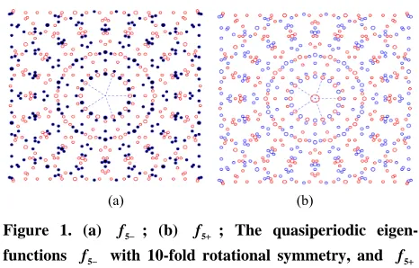
(with an:a0). Figures 1 and 2 show representations of

such eigenfunctions with n5 an resp Filled circles correspond to negatively scaled Dirac



1 2



det a a 1, _d _n_₇ _ectively.

 ’s, and unfilled cir les correspond to positively scaled Dirac and grida a_{1 2}_, is distinct from , then

 

1 2

,

grida a 

 

 ’s. The radius of ea circle is proportional to the c square root of the modulus of the scale factor for the corresponding

 

1 2, 1 2,

: grid_{a a} grid_{a a}

f x  x   x (31) ch

 . By construction

 

: grida a1 2,

 

grida a1 2,

 

f x  x   x (32) _,

are eigenfunctions of the Fourier transform operator associated with



1, 1

   , respectively. fn fn and fn fn .

 

     Quasiperiodic eigenfunctions of  on with

m-fold rotational symmetry.

2



3. Representation of Some Quasiperiodic

Eigenfunctions

Let

2 1 sin

n

  _ _

  (33)

for some n3, 4, , and let













T

cos 2 ,sin 2

k

a  k n k n

1,

(34)

where 0  k n be the vertices of a regular

gon

n with center at the origin. The parameter 

has been chosen so that (a) (b)



1



det ak ak 1 for each k1, 2, , n1. Thus

1 1

, ,

grida_k a_k gridQa Qa_k _k ,k 0,1, ,n 1

 _ _ _ _

Figure 1. (a) f₅ ; (b) f5 ; The quasiperiodic eigen- functions f5 with 10-fold rotational symmetry, and f5

[image:8.595.306.539.564.713.2]

(9)

(a) (b)

Figure 2. (a) f₇ ; (b) f7 ; The quasiperiodic eigen- functions f₇ with 14-fold rotational symmetry, and f7 with 28-fold rotational symmetry for the Fourier transform operator  with respectively = 1 , and = 1.

REFERENCES

[1] R. N. Bracewell, “Fourier Analysis and Imaging,” Kluwer Academic, New York, 2003.

http://dx.doi.org/10.1007/978-1-4419-8963-5

[2] L. Schwartz, “Theorie des Distributions,” Hermann, Paris, 1950.

[3] R. Strichartz, “A Guide to Distribution Theory and Fou- rier Transforms,” CRC Press, Inc., Boca Raton, 1994.

[4] B. Osgood, “The Fourier Transform and Its Applications,” Lecture Notes, Stanford University, 2005.

[5] D. W. Kammler, “A First Course in Fourier Analysis,” Prentice Hall, New Jersey, 2000.

[6] J. I. Richards and H. K. Youn, “Theory of Distributions: A Non-technical Introduction,” Cambridge University Press, Cambridge, 1990.

http://dx.doi.org/10.1017/CBO9780511623837

[7] M. J. Lighthill, “An Introduction to Fourier Analysis and Generalized Functions,” Cambridge University Press, New York, 1958.

http://dx.doi.org/10.1017/CBO9781139171427

[8] L. Auslander and R. Tolimieri, “Is Computing with the Finite Fourier Transform Pure or Applied Mathematics?” Bulletin of the American Mathematical Society, Vol. 1, 1979, pp. 847-897.

http://dx.doi.org/10.1090/S0273-0979-1979-14686-X [9] J. H. McClellan and T. W. Parks, “Eigenvalue and Eigen-

vector Decomposition of the Discrete Fourier Transform,” IEEE Transactions on Audio and Electroacoustics, Vol. 20, No. 1, 1972, pp. 66-74.

http://dx.doi.org/10.1109/TAU.1972.1162342

[image:9.595.59.285.85.200.2]