Munich Personal RePEc Archive
Interdependence in Multinational
Production Networks
Chen, Maggie
George Washington University
2009
Interdependence in Multinational Production Networks
Maggie X. Cheny George Washington University
January 2010
Abstract
The majority of multinational …rms today operate a multilateral production net-work. Most existing empirical analyses have, however, focused on …rms’ choice be-tween producing at home and investing overseas and assumed that a …rm’s decision to invest in a foreign country is independent of its locations in third countries. This paper examines the e¤ect of existing production network on multinationals’ entry decision. Using detailed French multinational subsidiary level data, the paper …nds strong evidence of horizontal and vertical interdependence across multinationals’ foreign production locations. There is, however, little evidence of horizontal in-terdependence between home-country production and foreign investment when the third-country e¤ects are taken into account, constituting a sharp contrast to the con-ventional emphasis. This result is robust to the various speci…cations and sensitivity analyses undertaken in the paper, and highlights the importance of investigating the causes and e¤ects of foreign direct investment in the context of multinational production network.
Key words: multinational …rm, production network, interdependence, entry de-cision, trade cost, input-output linkage
JEL codes: F23, D21
I am very grateful to Ron Davies, Jonathan Eaton, Peter Egger, Jim Markusen, Keith Maskus, Mike Moore, Andreas Waldkirch, Stephen Yeaple and participants of the 2008 Empirical Investigation of International Trade (EIIT) Conference, the 2009 Midwest International Trade Group Meeting, and the 2009 Econometric Society Summer Meeting for valuable comments and suggestions. Research funding from George Washington University Center for International Business Education and Research (CIBER) is also acknowledged.
1
Introduction
The majority of multinational corporations (MNCs) today operate a multilateral production network. An average French multinational, for example, invests in 3.8 foreign countries in 2007, with an increase of 0.93 country per …rm compared to 2005. The vast empirical literature of multinational …rms has, however, largely ignored the multilateral nature of MNC production and primarily focused on the relationship between home-country production and foreign investment. Most studies in the literature assume that a multinational …rm’s decision to invest in a foreign country isindependent of its existing production network in third countries, an assumption that is increasingly at odds as multinationals expand their production across foreign nations.
This paper addresses the above issue by examining the e¤ect of third-country production network on multinationals’ entry decisions. To achieve the goal, the paper employs a rich dataset that provides detailed information on French manufacturing …rms’ foreign subsidiaries in 2005 and 2007. For each subsidiary, the data reports the location, ownership status, and production activities. These information allows the paper to identify each individual …rm’s production network around the world and compare the structure of the network over time. They also enable the paper to establish intra-…rm linkage between subsidiaries, in particular, the input-output relationship between subsidiaries’ production activities. This makes it possible to distinguish the nature of interdependence between multinationals’ foreign subsidiaries.
Figure 1, for example, plots the geographic distribution of Renault’s global production net-work. Two observations emerge in this …gure. First, Renault owns subsidiaries in more than 10 countries outside of France. Second, Renault segments its production across its foreign production locations by producing components in countries such as Argentina, South Korea, and Spain (represented by the darker area) and performing end processes in countries such as Russia and Colombia (represented by the lighter area). These phenomenons are not exclusive to Renault, however. Figure 2 shows a similar pattern for another French multinational …rm, Essilor, which specializes in lens products. In fact, our data indicates that as of 2007 French multinational …rms have, on average, 0.72 upstream subsidiaries abroad (in which they produce intermediate inputs required for …nal-good production) and 2.49 downstream subsidiaries (in which they produce the …nal products). It is clear that multinationals’ investment decision can no longer be viewed as a choice between producing at home and investing abroad; it involves instead anetwork of vertically linked subsidiaries.
[Figures 1-2 about here]
…rms’ existing foreign subsidiaries is relatively high. We refer to this e¤ect ashorizontal inter-dependence. Second, multinationals tend to produce the …nal product in countries with better access to large export markets where the MNCs do not have downstream production. We label this e¤ect as the market potential factor. Third, there is a signi…cant interaction between up-stream and downup-stream subsidiaries. Speci…cally, multinationals tend to locate the …nal-good production in countries where the cost of importing intermediate inputs from the …rms’ existing foreign upstream subsidiaries is relatively low. Similarly, they are more likely to select coun-tries with better market access to the existing downstream subsidiaries as intermediate-input production locations. We refer to this type of interaction asvertical interdependence and show that it is not uniform across vertically linked subsidiaries. The interdependence increases in the extent of input-output linkage between subsidiaries as well as the size of market demand in downstream production locations.
In sharp contrast to the strong interaction between MNCs’ foreign production locations, there is little evidence of horizontal interdependence between multinationals’ production at home and new investment abroad. We …nd in the paper that evidence that would support the traditional argument — on the tradeo¤ between foreign investment and home-country production — be-comes insigni…cant once we take into account the third-country network factors. Instead, we observe a vertical interdependence. These results are robust to the various speci…cations and sensitivity analyses undertaken to address the bias of omitted variables and the potential endo-geneity of network factors. This deviation from the literature suggests that assuming away the interdependence between foreign production locations is likely to give rise to biased estimates on the relationship between home-economy performance and FDI activities and, more generally, biased understanding of the true causes and e¤ects of FDI. It calls for a reconsideration of the conventional speci…cation to take into account the e¤ect of third-country network. The …ndings also convey an important message to host-country policy makers that seek to in‡uence the in‡ow of foreign investment: FDI in‡ow to third countries can a¤ect a country’s ability to attract multinationals. The e¤ect can be either positive or negative dependent on the linkage of FDI ‡ows.
This paper is closely related to a growing theoretical literature, led by Yeaple (2003a), Ekholm, Forslid and Markusen (2007), and Bergstrand and Egger (2008), that applies FDI modeling to a three-country framework. These studies build on the seminal work of Markusen (1984) and Helpman (1984) and in‡uential empirical contributions by Brainard (1997), Carr, Markusen and Maskus (2001), Yeaple (2003b), Helpman, Melitz and Yeaple (2004), and Hanson, Mataloni and Slaughter (2005), who point out the two main motives for multinationals to invest abroad are market access and comparative advantage.1 Yeaple (2003a), Ekholm, Forslid and Markusen (2007), and Bergstrand and Egger (2008) show that the combination of the market-access and comparative-advantage motives can lead to export-platform FDI, where a
multinational …rm invests in a host country with the intention to serve third nations via exports from the host country. This prediction suggests that multinationals’ investment decision cannot be viewed as a binary choice between exporting from home and investing abroad; it engages other, third nations.
The majority of the empirical literature has, however, not taken into account the third-country e¤ect, much less the interdependence between multinationals’ foreign production loca-tions. The following few studies took the step to examine the determinants of export-platform FDI. Head and Mayer (2004) show that third-country market demand plays a signi…cant role in a country’s ability to attract multinational …rms. They …nd that Japanese multinationals are more likely to locate their production in regions proximate to large markets. Baltagi, Egger and Pfa¤ermayr (2007) consider a broader set of third-country characteristics, and …nd that most of the characteristics exert a signi…cant e¤ect on the level of U.S. outbound FDI even though there is no conclusive evidence on export-platform or vertical FDI. Chen (2009) examines how a host country’s preferential trade agreement with third nations can a¤ect the country’s receipt of FDI and …nds that countries integrated with large markets tend to experience an increase in total and export-platform investment. She also shows that the e¤ect is especially strong for labor-abundant countries, but at the expense of the labor-scarce preferential trading partners.
Blonigen, Davies andet al. (2007) is among the …rst to investigate cross-country interdepen-dence in FDI. Using U.S. outbound FDI data, they examine how investments in third countries a¤ect a country’s receipt of FDI from the U.S. They …nd that the results are sensitive to the sample of host countries examined: the third-country e¤ect can be either insigni…cant or of reverse signs. There is some evidence of negative interdependence across proximate host coun-tries — a result that is consistent with the export-platform FDI theory — but mainly among European OECD members. They also …nd that including third-country FDI does not alter the estimated e¤ect of traditional FDI determinants.
intra-…rm interdependence leads to sharply di¤erent …ndings than previous studies: the estimated horizontal interdependence between FDI and home-country exports disappears once we include third-country network variables. This departure from previous …ndings is not surprising given the data used there is not equivalent to an individual …rm’s investment decision.
The rest of the paper is organized as follows. In Section 2, we examine the geographic attributes of French MNC production networks. In Section 3, we use a simple three-country theoretical framework to provide a motivation for the empirical analysis. We then describe the econometric methodology in Section 4 and data sources in Section 5. We present the main econometric results in Section 6 and several sensitivity analyses in Section 7. The paper concludes in Section 8.
2
Attributes of French MNC production networks
We employ a dataset of French manufacturing MNCs for our empirical analysis. In this section, we …rst take a look at the attributes of French MNC production networks. Figures 3 plots the distribution of French multinational …rms in 2005 and 2007 by the number of countries in which investments occur. The majority of French MNCs concentrate their foreign production activities in 3 or more countries in 2007 while some spread to as many as 63. Comparing 2007 with 2005, there is a signi…cant expansion in the size of network with an average increase of 0.93 per …rm. A large fraction of foreign production locations comprises downstream subsidiaries, i.e., subsidiaries that engage in …nal-good production.2 The average number of countries in which …rms own downstream subsidiaries is 2.49, signi…cantly greater than the average number of countries in which …rms have upstream production locations.
[Figure 3 about here]
Now we examine the geographic density of each production network. In Figure 4, we plot the level of distance between each pair of subsidiaries owned by the same French MNCs. As shown in the graph, the closest two subsidiaries are 66 kilometers apart (located in Austria and Slovakia) and the furthest pair is 19,845 kilometers apart (in Estonia and New Zealand). The majority of subsidiaries are within 6,126 kilometers, while the average distance is about 6,000. The graph also indicates that a large percentage of French MNC subsidiaries are either clustered in neighboring countries (such as EU members) or located relatively distant from each other. This is further con…rmed at the multinational …rm level where we calculate the average subsidiary distance for each French MNC: While a signi…cant fraction of French multinationals have a dispersed subsidiary network, many of them concentrate their subsidiaries geographically. We then compare the distance between downstream production locations (owned by the same French MNCs) with the distance between vertically linked subsidiaries. As shown in Figure 5,
the former tends to be greater than the latter as expected. Multinationals tend to duplicate their …nal-product production in countries that are geographically distant from each other. But they build their upstream and downstream subsidiaries in proximate locations.
[Figures 4-5 about here]
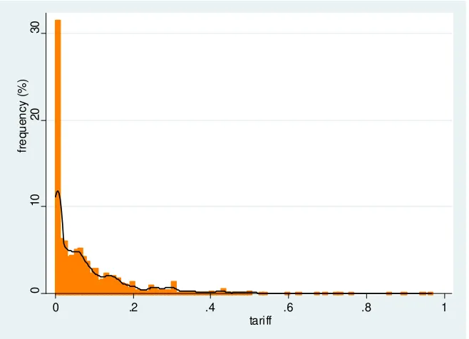
The above observations similarly apply to tari¤s. In Figure 6, we plot the level of tari¤ between each pair of subsidiaries on the subsidiaries’ primary good. It is shown that more than 30 percent of subsidiary pairs do not have tari¤ between each other and more than 50 percent have 7% or lower tari¤ rates. This is also con…rmed at the parent …rm level: More than 15 percent of French MNCs locate their subsidiaries in countries where tari¤s have been removed for each other and 50 percent face an average of 6% or lower tari¤ when exporting from one subsidiary to another. This suggests that French MNCs are not always driven by the tari¤-jumping motive when they choose their foreign production locations; a large percentage of them invest in countries where they can export to without paying tari¤. This becomes more clear when we compare in Figure 7 the tari¤ between downstream production locations (on …rms’ …nal good) and the tari¤ of importing intermediate inputs from upstream locations. The former is signi…cantly higher than the latter, suggesting tari¤s motivate …rms to expand their production horizontally but discourage them from building vertical production network.
[Figures 6-7 about here]
3
Theoretical motivation
As a prelude to the empirical analysis, we consider a stylized theoretical framework in this section and provide a motivation for the empirical hypotheses.
3.1 General setup
Suppose the world consists of N countries N =f1;2; :::; Ng. The representative consumer in each country allocates a certain amount of her expenditure, denoted as Ij (j 2 N), to the
industry of di¤erentiated products. Within this industry, the consumer has a utility function with constant elasticity of substitution (CES). Maximizing the CES utility function subject to the consumer’s expenditure level yields the consumer demand function for each representative varietyqij =Yjpij ;whereqij is the quantity of the di¤erentiated product produced by …rms in
countryiand sold to destination country j,Yj Ij=Prp1rj is the demand level in countryj
withrrepresenting the set of varieties,pij the price of this product, and the constant elasticity
of substitution. Note thatpij = ij pi, wherepi is countryi’s product market price and ij >1
Each …rm produces a di¤erent brand of the di¤erentiated product. Given the interest of this paper, we assume that country 1’s …rms can produce their …nal good in any of the other countries while the other countries’ …rms produce only at home and serve the foreign markets via exports. Firms must pay a plant-level …xed costF for each …nal-good production location. They must also produce one unit of intermediate input for each unit of …nal product.3 Like
the …nal product, country1’s …rms can produce the intermediate input in any of the countries. For simplicity, we assume that the plant-level …xed cost for intermediate-input production, G, is su¢ciently large such that …rms would build their upstream production in only one location.4
We also assume that the upstream subsidiary will sell the inputs to the downstream subsidiaries atmk ki, where mk is the marginal cost of producing the intermediate input and ki is the cost
of exporting the intermediate input from country kto countryi.
Now let di be an indicator variable that equals to 1 if the …rm locates the downstream
production in country i and similarly ui be an indicator variable that identi…es the existence
of upstream production location. We can then characterize each …rm’s production network as g fdi; uig, where i 2 N. Based on the observed production network, we de…ne a …rm
as a national …rm if there is no subsidiary abroad, and a multinational if there is at least one foreign subsidiary. We also let Nd(g) = fi2 N :di = 1g denote the set of countries in which
the …rm has downstream production and Nu(g) = fi2 N :ui = 1g the set in which the …rm
has upstream production. We use nd(g) and nu(g) to represent the cardinality of the two sets
respectively.
In the rest of this section, we examine …rms’ decision to undertake horizontal and vertical investments in a given production network. First, we note at pro…t maximization each …rm will set the price at
pi =
(ci+mk ki)
( 1) ; (1)
where ci is the marginal cost of producing the …nal good in country i. This implies that the
operating pro…t the …rm will earn by producing the intermediate input in country k and …nal good in countryiand selling to destination country j, i.e., g=fdi = 1; uk= 1g, is
ij(g) =
1 1
ci+mk ki
1
ij Yj: (2)
It is clear that ij is an increasing function of countryj’s demand (i.e.,Yj) and a decreasing
3Given this paper’s focus on intra-…rm linkages, we do not consider here the option of purchasing intermediate
inputs from una¢liated suppliers. The latter possibility and its role in …rms’ location decision is an interesting reseach question in its own right and has a large scope for future empirical research. For seminal theoretical studies in this area, see, for example, Krugman and Venables (1996), Venables (1996), and Puga and Venables (1997). The empirical analysis of this paper attempts to control for these factors using host-country and …rm …xed e¤ects as …rm-level data that identi…es intermediate-input suppliers is largely missing.
4While this assumption is roughly in alignment with the data which shows French multinationals have, on
function of the …nal good marginal cost (i.e., ci) and the trade cost to ship the …nal good from
country i to country j (i.e., ij). Furthermore, because production consists of two stages, ij
also decreases in the marginal cost of producing the intermediate input (i.e., mk) as well as the
trade cost of shipping the input to the …nal good production location (i.e., ki).
Now suppose the …rm has chosen Nd(g) as the set of locations to produce the …nal good
and country kas the location to produce intermediate inputs, i.e.,Nu(g) =k. The total pro…t
function will then be
(g) = X
i2Nd(g)
1 1
ci+mk ki
1
Yi (3)
+ X
j2N nNd(g) max
i2Nd(g)
"
1 1
ci+mk ki
1
ij Yj #
nd(g)F G:
In this equation, the …rst term represents the operating pro…t from domestic sales (in countries with has downstream production), the second term represents the operating pro…t from export sales (in markets without downstream production), and the last two the …xed costs of down-stream and updown-stream production (which increases as …rms expand the number of production locations). Note that the export pro…t depends on the choice of export-platform countries, i.e., the downstream production locations in Nd(g) from which the …rm exports to the other
markets. Firms will strictly prefer location con…guration g tog if and only if
(g )> (g): (4)
3.2 Downstream location decision
Given our goal to examine …rms’ investment decision in a given production network, suppose the current production network comprises a downstream plant in countryei and an upstream plant in country ek, i.e., g0 = fdei = 1; uek = 1g. We …rst look at the decision to build a new
downstream production subsidiary in country i, i.e., di. If di = 1, the production network
will move from g0 tog1 =fdi=dei = 1; uek= 1g.
Firms will build a downstream subsidiary ini if and only if
(g1)> (g0): (5)
Given equation (3), we can simplify the above condition to
(ci+mek eki)
1 M
i > ei( eii Yi+M e
ei) + F; (6)
whereMi Yi+Mie=Yi+ P
includes country i’s domestic market size Yi and the size of export markets Mie in which the
…rm does not have downstream production, and ei (cei+mke ekei)1 .5 Let e
ki mek=ci denote
the extent of vertical linkage between intermediate input and …nal good; the above expression can be re-written as:
c1i (1 + eki eki)1 Mi> ei( eii Yi+M e
ei) + F: (7)
As monotonic transformations and terms such as ei and Me
ei do not a¤ect the ordering of
host countries (i), we simplify condition (7) (and take natural logs on both sides) to obtain a simple and intuitive empirical speci…cation:
Pr [ di = 1jg0] = (8)
[ d1lnci+ d2lnYi+ udln(1 + eki eki)
| {z }
vertical
+ md lnMi
| {z } market potential
+ ddln eii
| {z } horizontal
+"]:
In this speci…cation, Pr [ di = 1jg0] represents each …rm’s probability to build a new
down-stream production location in countryigiven its existing production network g0 and [:]is the
cumulative probability function. The terms ln(1 + eki eki) and ln eii represent the trade costs to import from the …rm’s existing upstream and downstream production locations respectively, capturing thevertical and horizontal interdependence in the network. The variablelnMi
repre-sents country i’s market potential given …rm’s downstream production network. The residual"
captures all the remaining factors including ei and Me
ei, which comprise attributes of the …rm’s
existing production location and are invariant with countryi’s attributes. We control for these factors with …rm dummies in the empirical analysis.
We expect, based on the model, that the e¤ect of host-country variables satis…es d1 <0and
d2 >0. The e¤ect of existing production network varies with the nature of the subsidiaries.
We expect the e¤ect of vertically linked subsidiaries to satisfy ud <0, i.e., …rms have a greater incentive to build downstream subsidiaries where the cost of importing intermediate inputs is low, especially when the vertical linkage between upstream and downstream production, i.e.,
eki, is large. The expected e¤ect of existing downstream network is d
d>0, i.e., …rms are more
likely to expand horizontally when the trade cost of importing …nal goods is relatively high. The host-country market potential is predicted to have a positive e¤ect, implying md >0.
5The above condition assumes that …rm will choose the new downstream subsidiary as the export platform to
3.3 Upstream location decision
Now consider …rm’s upstream location decision. Given networkg0 (where dei = 1; uek= 1), …rm
will build a new upstream production subsidiary in country kand move to network g2=fdei=
1; uk= 1gif and only if
(g2)> (g0): (9)
Given equation (3), this is equivalent to
(cei+mk kei)
1 (c
ei+mek ekei)
1 M
ei>0: (10)
It can be further transformed to
m1k 1
kei
+ kei
1
> ei; (11)
where kei mk=cei and ei (cei+mek ekei)1 .
Based on the above condition, we obtain the following simpli…ed speci…cation to examine …rms’ decision to build upstream subsidiaries:
Pr [ uk= 1jg0] = [ ulnmk+ duln kei
| {z } vertical
+"]: (12)
In this expression,Pr [ uk = 1jg0]denotes …rm’s probability to build a new upstream production
location in country k given its existing production network g0. We expect that u < 0 and d
u < 0 (i.e., …rms have greater incentives to produce the intermediate input in countries with
relatively better access to the …rms’ existing downstream production locations, i.e., low kei).
4
Econometric framework
We now describe the econometric framework adopted in the empirical analysis. Following equa-tions (8) and (12), we consider the following speci…caequa-tions:
downstream : Pr [ dt= 1] =Xt 1 d (13)
+ dd Wd;td 1 dt 1+ ud Wd;tu 1 ut 1+ md lnMt 1+ d;t
uptream : Pr [ ut= 1] =Xt 1 u+ ud Wu;td 1 dt 1+ u;t: (14)
In the above equations, dtand utare two vectors of observations of the two binary dependent
variables which represent, respectively, each …rm’s decision to build downstream and upstream subsidiary in a given country, Xt 1 is a matrix of observations of lagged exogenous variables,
including (i)Wd
d;t 1 dt 1 (horizontal interdependence) wheredt 1 fdit 1(a)grepresents each
…rm’s downstream production locations in the lagged period, (ii)Wu
d;t 1 ut 1 and Wu;td 1 dt 1
(vertical interdependence), whereut 1 fuit 1(a)grepresents each …rm’s upstream production
locations in the lagged period, and (iii)Mt 1 Wd;tm 1 (1 dt 1)(market potential). Our goal
is to estimate d
d, ud, md and du along with d and u.6
We now de…ne the four weighting matrices, Wd
d;t 1,Wd;tu 1,Wd;tm 1 and Wu;td 1, used in the
model. First, consider four N N matrices !d
d;t 1(a), !ud;t 1(a), !md;t 1(a), and !du;t 1(a) for
each …rm in the sample (where adenotes the …rm and N the number of countries). The cells in !d
d;t 1(a) are de…ned based on equation (8) and given by
!dd;ijt 1(a) = ln jit 1(a); (15)
where i; j= 1; :::; N and jit 1(a) >1 is the trade cost …rm aincurs when importing the …nal good from countryj to countryi. If …rmaindeed produces the …nal product in country j, the higher this cost, the more incentive …rm ahas to invest in countryi.
Similarly, the cells in !u
d;t 1(a) are given by
!ud;ijt 1(a) = ln 1 + j(a) jit 1(a) ; (16)
where j(a) is the input-output coe¢cient between the good produced by …rm a in country j
and its …nal good and jit 1(a) is the trade cost for …rm a to import the good produced in countryjto country i. If …rmaindeed produces in countryj and the good produced serves as an intermediate input for a’s …nal good (i.e., j(a)>0), a greater trade cost to import from j
would lower …rma’s incentive to locate downstream production in countryi.
Next, following Section 3.2, we de…ne Mi Pj(1 dj)Yj= ij and the cells in!md;t 1(a)as
!md;ijt 1(a) =Yjt 1= ijt 1(a); (17)
where Yjt 1 is the market demand in country j and ijt 1(a) is the trade cost …rm a would
incur when exporting the …nal good from country i to country j. Each cell in !m
d;t 1(a) thus
captures country i’s export market potential in countryj. Finally, the cells in !d
u;t 1(a) are de…ned based on equation (12):
!d
u;ijt 1(a) = ln ijt 1(a); (18)
6We do not consider in this paper the potential contemporaneous correlation between entries for two reasons.
where ijt 1(a) is the trade cost for …rm a to export intermediate inputs from country i to countryj. Ifahas a downstream production location inj, this trade cost is negatively correlated witha’s incentive to produce the intermediate input ini.
Given!d
d;t 1(a),!ud;t 1(a),!md;t 1(a)and!du;t 1(a), we can construct the aggregate weighting
matrices, Wd
d;t 1, Wd;tu 1, Wd;tm 1 and Wu;td 1. These aggregate matrices consist of !dd;t 1(a),
!u
d;t 1(a), !md;t 1(a) and !du;t 1(a) respectively along the diagonal and 0 everywhere else. For
example, Wd
d;t 1 is anN K N K matrix given by
Wd;td 1 =
2 6 6 6 6 6 6 4 !d d;t 1(a1)
nd;t 1(a1) 0 0 0
0 !
d d;t 1(a2)
nd;t 1(a2) 0 0
0 0 . .. 0
0 0 0 !dd:t 1(aK)
nd;t 1(aK)
3 7 7 7 7 7 7 5 (19)
where a1; a2; :::; aK represent the set of …rms in the sample (with K = 1698) and N represents
the number of host countries and equals to99. Note we scale!d
d;t 1(a),!ud;t 1(a)and!du;t 1(a)
with the …rm’s (downstream and upstream) production network size, i.e.,nd;t 1(a1),nu;t 1(a1)
and nd;t 1(a1) respectively. The purpose of doing this is to estimate average interdependence
across subsidiaries.
Finally, we include a …rm …xed e¤ect throughout the empirical analysis to control for all …rm-speci…c factors such as factor intensities and the aggregate attributes of existing subsidiaries.7 The use of …rm dummies allows us to focus exclusively on the cross-country interaction within each multinational’s production network.
5
Data
The dataset employed in this paper is obtained from BvDEP AMADEUS, a comprehensive database that contains the …nancial and subsidiary information of public and private European …rms. AMADEUS is collected by information providers at each national o¢cial public body (e.g., Institut National de la Propriete Industrielle (National Institute for Industrial Property) in the case of France) and has a particularly good coverage for countries including France, which partly motivated the use of French …rms for this analysis.
The dataset reports French multinationals’ subsidiary activities in 99 host countries in 2005 and 2007.8 It is compiled from two editions of AMADEUS that were published in 2006 and
7To avoid the incidental parameter problem that would arise with …xed-e¤ect Maximum Likelihood Estimators,
we adopt linear-probability model in Section 6. We also considered excluding …rm …xed e¤ect and using probit and logit models while controlling for …rm characteristics such as capital intensity and productivity. The main results remain largely similar and are available upon request. We did not adopt conditional logit model because it would drop all multinational …rms that did not incur any entry from the empirical analysis.
2008 respectively.9 For each multinational …rm, the data lists not only the subsidiary locations but also the primary product, sales, assets and employment of each location.10 There are in
total 1,698 French multinational …rms in the dataset. These …rms invest in on average 2.88 host countries in 2005 and 3.81 countries in 2007. The average increase in the number of invested countries is 0.93.11
As discussed in Section 3, we distinguish two types of subsidiaries. To do so, we follow the methodology introduced in Alfaro and Charlton (forthcoming). First, we identify subsidiaries that engage in …nal-good production. To do so, we compare each subsidiary’s primary prod-uct with the parent …rm’s primary and secondary prodprod-ucts, all of which are reported at NACE 4-digit level.12 If the subsidiary’s primary product is listed as one of the parent …rm’s …nal prod-ucts, it is considered as a downstream production location. We also identify subsidiaries that engage in upstream production. This is determined by examining the input-output relationship between the subsidiary’s primary product and the parent …rm’s …nal products. A subsidiary is considered as an upstream production location if the direct requirement of the subsidiary’s primary product in the parent …rm’s …nal-product production exceeds a threshold value.13 This direct identi…cation of downstream and upstream subsidiaries has been generally absent in the literature, with the exception of Alfaro and Charlton (forthcoming), mainly because of the lack of information on subsidiary-level activities.
According to our de…nition, we …nd the average number of countries in which French multi-nationals have downstream subsidiaries is 2.49 whereas the number of countries with upstream subsidiaries is around 0.72.14 More than 75 percent of newly established subsidiaries between 2005 and 2007 are downstream production locations, suggesting that …rms are more inclined to expand horizontally than vertically.
Following Section 4, we use three subsidiary-level variables to construct the various weighting matrices needed to de…ne existing network characteristics. These variables include (i) the distance between each pair of host countries (as a proxy for transport cost), (ii) the tari¤ rates between each pair of host countries on parent …rms’ …nal products and intermediate inputs produced overseas, and (iii) the input-output coe¢cient between the parent …rm’s …nal products and the subsidiary’s primary good. We obtain the distance data from the CEPII distance
9AMADEUS does not directly report time series on subsidiary data. To obtain that information, one needs
to acquire di¤erent editions of AMADEUS that were published in di¤erent years.
1 0The coverage of sales, assets and employment data is not as complete as the location information.
1 1It is worth noting that there are very few exits (i.e., subsidiary shut-downs) in the dataset. Nearly all the
subsidiaries that existed in 2005 are active in 2007.
1 2AMADEUS reports both primary and secondary products for parent …rms. We take into account both in
our de…nition of downstream and upstream subsidiaries.
1 3The paper has considered di¤erent threshold values and found the results relatively similar. The results
presented in the following sections are obtained based on the threshold value 0.1. We also weigh each upstream subsidiary with its input-output coe¢cient.
1 4Less than 20 percent of subsidiaries belong to neither cateogries and engage in activities such as wholesale
database and tari¤ data from the WITS. The tari¤ data are applied tari¤ rates measured at NACE 4-digit level and re‡ect preferential tari¤ rates between host countries. We use the input-output table from the 2002 U.S. Bureau of Economic Analysis (BEA) benchmark survey. This I-O table is more disaggregated than the alternatives including the I-O table from the INSEE (and other available national sources).
In addition to the …rm network variables, we take into account FDI determinants that have traditionally been emphasized in the literature. First, we include several conventional variables used to capture the trade cost between home and host countries. Existing studies point out that multinationals have a greater incentive to invest in countries that require larger trade costs to export the …nal goods from home. To examine the importance of this motive, we include the distance between a potential host and France and tari¤ rates set by host countries on France in each multinational …rm’s primary …nal product category.15 The hypothesis predicts a positive parameter on both variables: the higher the transport cost and host-country tari¤ for …rms to export the products from home, the more likely the …rm will produce the product inside the host country. In addition to the above market access variables, we also include host-country domestic market size, measured by real GDP. Multinationals that are attracted by the host-country local market size are expected to have a greater probability of investing in larger countries.
We also control for multinationals’ comparative advantage motive. Speci…cally, we take into account host countries’ marginal cost of production by including each host country’s real unit labor cost. This data is aggregated from the industry level where each industry is weighed by its output share. The labor cost and output data are available from the World Bank Trade and Production Database. Furthermore, we include the tari¤ rate France sets on the host-country exports. The expectation is that multinationals seeking to export their products back to France would be adversely a¤ected by this tari¤.
Finally, we take into account various measures of investment costs. First, we control for host countries’ tax policy using the maximum corporate tax rate, available from the U.S. O¢ce of Tax Policy Research.16 Second, we include the costs of starting a business, available from the World Development Indicators, as a proxy for entry cost. Third, we use the distance between France and the host country as a proxy for …xed cost of investment, with the expectation that subsidiaries located in remote markets are likely to require a larger …xed cost such as the cost of monitoring. Note all the explanatory variables are measured with the 2005 data. Table A.1 describes the source and summary statistics of the variables.17
1 5We also used the average tari¤ rate imposed on the …rm’s primary and secondary products. The results were
qualitatively similar.
1 6Ideally, we would like to use the applied corporate tax rate in each host country. But this data consists of a
large number of missing values for the countries in our sample.
1 7In the empirical analysis, we also consider using a country …xed e¤ect to control for omitted host-country
6
Empirical evidence
We now turn to the econometric analysis and examine the e¤ect of existing production networks on multinationals’ entry decision. We proceed by …rst estimating equations (13) and (14) with only conventional explanatory variables, i.e., excluding the e¤ect of third-country locations and assuming dd= 0, ud = 0, md = 0, and du = 0.
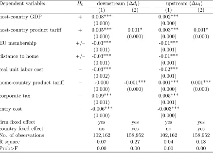
Excluding network e¤ects
The results are reported in Table 1. We …nd the e¤ect of included explanatory variables is largely consistent with the existing literature when no third-country factors are taken into account.18 First, …rms exhibit a signi…cant market-access motive that is in alignment with the literature. They are more likely to build …nal-good production in countries with a larger GDP. They also have a greater incentive to enter countries that set a higher tari¤ on the imports of their …nal products from France. The parameter of EU membership is also consistent. Firms are more likely to choose FDI instead of export in countries outside the EU. The e¤ect of distance is negative, a …nding that has been shown in previous studies and explained by the role of distance in raising the …xed cost of investment.
The evidence also indicates a signi…cant comparative advantage motive. Countries with a lower unit labor cost attract more multinationals to build downstream production. Investment costs also exert a signi…cant e¤ect on multinationals’ entry decision. A larger cost of starting business is associated with a lower probability of attracting multinational …rms. The sign of the corporate tax parameter is inconsistent with expectation, however. This can be a result of the tax measure included in the paper. The corporate tax data used here reports each host country’s maximum corporate tax rate and does not necessarily capture the rate applied to multinational …rms. The latter information is not systematically available and would reduce the sample size substantially.
[Table 1 about here]
In the fourth column of Table 1, we include a host-country …xed e¤ect to control for all unobserved host-country characteristics. We …nd the e¤ect of host-country tari¤ set on France remains signi…cant and positive. This suggests controlling for country-level attributes does not change the estimated e¤ect of the conventional market access variable. The parameter of home-country tari¤ also becomes signi…cant: A higher tari¤ to export the …nal product back to France lowers multinationals’ incentive to produce the good abroad. This result is consistent with the comparative advantage motive hypothesis: Some French multinationals serve their home country from foreign production location and are adversely a¤ected by home-country tari¤.
1 8The
H0 column in Table 1 (and the following tables) summarizes the hypotheses on the e¤ect of explanatory
Next we examine multinationals’ upstream location decision. As shown in the last columns of Table 1, the results are largely similar. Countries with a larger GDP and a higher tari¤ have a greater probability to attract multinationals. Those that are relatively remote from France and have a higher real unit labor cost or a higher entry cost are less likely to become upstream production locations. A result that is not expected analytically is the positive e¤ect of French tari¤. A higher tari¤ to export the …nal product back to France motivates French …rms to move upstream production overseas. Again, controlling for unobserved host-country attributes with host-country dummies does not change the estimated e¤ect of host- and home-country tari¤s on each other.
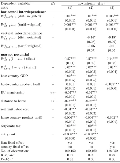
Including network e¤ects
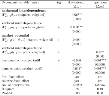
Now let us take into account the potential e¤ect of foreign production network. Table 2 reports the estimates obtained for the downstream equation in (13). The table indicates strong evidence of horizontal and vertical interdependence in multinationals’ foreign production network. First, multinationals are signi…cantly more likely to build downstream production in countries that are relatively distant from the …rms’ existing downstream locations. A 100-percent increase in third-country distance raises the probability of entry by 0.6 100-percentage point or equivalently 60 percent.19 This result similarly applies to tari¤. The incentive to enter a host country rises in the tari¤ of importing …nal good from the existing locations. Export-market potential also plays a signi…cant role. Multinationals have a greater probability to produce the …nal product in countries with a large export potential. This points out the signi…cance of export-platform FDI, in which multinationals use host countries as the platform to supply third countries — in particular, the third countries where multinationals do not have downstream production activities present. These …ndings remain robust after we include host-country …xed e¤ect and control for all host-country speci…c attributes.
[Table 2 about here]
The e¤ect of the conventional market access variables is a¤ected, however, by the consider-ation of downstream production network. As seen in Table 2, the parameter of host-country tari¤ on France becomes statistically insigni…cant when the third-country variables are taken into account. This constitutes sharp contrast with Table 1, where the evidence suggests a horizontal interdependence between foreign production and home-country exports: Market ac-cess from home has a signi…cant e¤ect on multinationals’ location choice. This change in the results suggests that it is not adequate to focus exclusively on the home-host interdependence. As multinationals’ production network expands over time, there is increasing interdependence across foreign production locations. The choice of where to invest is no longer conditional
on the tradeo¤ between FDI and exporting from home alone; it has become a more complex decision involving third countries. Ignoring the third-country network e¤ect is likely to give rise to biased estimates on the relationship between the performance of the home economy and FDI activities and, more generally, biased understanding of the true causes and e¤ects of FDI.
In column (2) of Table 2, we take into account the e¤ect of existing upstream production network. The results there show that the role of trade cost is reversed when there is a vertical linkage between foreign production locations. Multinationals are motivated to cluster vertically linked subsidiaries in proximate countries. For example, countries that are 100-percent farther to the multinationals’ existing upstream locations have a 0.1-percentage-point (equivalently 10 percent) lower probability to attract multinationals. This result suggests that upstream FDI in neighboring countries can trigger an increase in downstream FDI.
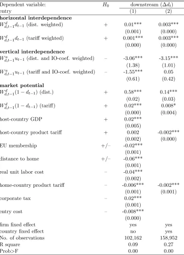
The e¤ect of upstream production network also increases in the extent of vertical linkage, as shown in Table 3. Here, we interact the trade cost of importing intermediate inputs with the input-output coe¢cient with respect to the multinationals’ …nal product. The parameters indicate that the incentive to cluster production stages is especially large when there is a strong vertical linkage. These results, again, are not sensitive to the use of host-country dummies.
[Table 3 about here]
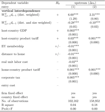
Now we proceed to examine multinationals’ upstream entry decision. As shown in Table 4, we …nd, again, signi…cant evidence of vertical interdependence. Multinationals tend to build upstream production locations in countries that are relatively proximate to the existing downstream locations. This is especially true when the downstream country has a relatively large market potential. These results re‡ect …rms’ incentive to reduce intra-…rm trade costs and build a geographically concentrated network of vertically linked subsidiaries.
[Table 4 about here]
7
Sensitivity analysis
7.1 Alternative weighting matrices
So far we have used distance and tari¤ to capture the extent of trade cost. While these two variables possibly represent the most prominent forms of trade barriers, they do not capture all the trade costs faced by multinationals. We hence consider in this section an alternative measure in the construction of weighting matrices. Speci…cally, we use disaggregate trade ‡ows as a proxy for host countries’ openness toward one another.
For example, when estimating …rm a’s downstream entry decision in country i given its existing downstream production location inei, we use the import value of countryifrom country
to countryei. Countries that are relatively open to the multinational’s existing downstream locations are less likely to be selected as new hosts. We also obtain country i’s import from countryekwhere …rmahas an upstream subsidiary (in the category of the subsidiary’s primary good). The hypothesis here is that multinationals are more likely to produce the …nal product in countries that are relatively more accessible from the …rms’ existing upstream locations. Finally, we use country i’s exports to all the third countries where …rm a does not have downstream production (in a’s primary …nal product) to construct i’s export market potential. To avoid endogeneity, we use trade data in 2005 which is available from COMTRADE.20
Table 5 reports the results obtained with trade-weighted network variables. The evidence indicates signi…cant and consistent horizontal and vertical interdependence across multination-als’ foreign subsidiaries. Multinationals have a particularly strong incentive to expand their downstream production in countries that import relatively less from their existing third-country downstream locations. They are also motivated to choose countries where there are large trade in‡ows from the …rms’ existing upstream subsidiaries.
[Table 5 about here]
When examining multinationals’ upstream entry decision, we take into account each host country’s market access to the …rms’ existing downstream locations. Speci…cally, for each multinational …rm aand and host countryi, we obtain i’s average export value to all the third countries where …rmaengages in …nal-stage production. Ideally, we would like to use the export of the subsidiary’s primary good, but this information is only observable for countries that have been selected as production locations. The counterfactual information is not available for those that were not chosen. As a result, we use each host country’s average export in manufacturing industries to construct the country’s market access. The results are reported in the last two columns of Table 5. There is a clear and signi…cant motive to locate vertically linked subsidiaries in countries with close trade relationships.
7.2 Endogeneity of network variables
In this sub-section, we address the potential endogeneity that can arise with the network vari-ables. So far we have used lagged location variables, i.e.,dt 1 and ut 1, to construct measures
of existing production networks. While the time lag between these variables and the dependent variables, i.e., dtand ut, and the control of …rm …xed e¤ect helps establish the causal e¤ect,
the former can still be endogenous because of the serial autocorrelation in the residuals, t. To
address this issue, we adopt a two-stage instrumental variable approach. In this approach, we use W Xt 1, where W represents Wd;td 1, Wd;tu 1, Wd;tm 1 or Wu;td 1 and Xt 1 is a matrix of
lagged host-country attributes, as potential instruments for the network variables.
Formally, we estimate:
downstream : Pr [ dt= 1] =Xt 1 d (20)
+ d
d Wd;td\1dt 1+ ud Wd;tu\1ut 1+ md ln\Mt 1+ d;t
uptream : Pr [ ut= 1] =Xt 1 u+ du Wu;td\1dt 1+ u;t; (21)
where
\
Wd
d;t 1dt 1 = E
h
Wd;td 1dt 1jWd;td 1Xt 1
i
\
Wu
d;t 1ut 1 = E Wd;tu 1ut 1jWd;tu 1Xt 1 (22)
\
lnMt 1 = E[lnMt 1jlnWd;tm 1Xt 1]
\
Wd
u;t 1dt 1 = E
h
Wu;td 1ut 1jWu;td 1Xt 1
i
:
The results are reported in Table 6. We …nd that most parameters remain qualitatively similar after we correct for the potential endogeneity of network variables with the exception of export market potential. We continue to observe signi…cant horizontal and vertical interde-pendence across multinationals’ foreign production locations.
[Table 6 about here]
8
Conclusion
This study is one of the …rst attempts to estimate the interdependence in multinationals’ global production network. Using a detailed French multinational subsidiary dataset, the paper …nds, for the …rst time, strong evidence of horizontal and vertical interaction between MNCs’ foreign production locations. These results complement existing contributions where evidence of in-terdependence, obtained with aggregate FDI data, has been ambiguous. Here we show that third-country subsidiaries exert a signi…cant e¤ect on French multinationals’ entry decision, in both downstream and upstream productions. But the e¤ect varies considerably with the linkage of subsidiaries. Multinationals are more likely to expand horizontally when the trade cost of importing …nal products from existing downstream subsidiaries is relatively high. But they tend to locate vertically linked subsidiaries in countries with low intra-…rm trade costs, espe-cially when there is a strong input-output relationship. These results are robust to the choice of weighting matrices used in the econometric model and the control of potential endogeneity in the network variables.
placed on the horizontal linkage between home- and host-country production. This departure can be explained by the assumption made in most previous studies that views a …rm’s decision to invest in a foreign country as independent of its locations in third nations, even though the majority of multinationals today operate a multilateral production network.
This paper conveys important policy implications for both FDI home and host countries: It is crucial to analyze the causes and e¤ects of FDI in the context of global production network. As shown in the paper, assuming away the interdependence between foreign production locations is likely to over-estimate the substituting relationship between home-country production and foreign investment. It would also fail to account for the spillovers between FDI ‡ows, including, for example, the e¤ect of FDI in‡ows to third countries on a host country’s ability to attract multinational …rms.
References
[1] Alfaro, Laura and Andrew Charlton. (forthcoming) "Intra-Industry Foreign Direct Invest-ment".American Economic Review.
[2] Baltagi, Badi H., Peter Egger, and Michael Pfa¤ermayr. (2007) “Estimating Models of Complex FDI: Are There Third-Country E¤ects?”.Journal of Econometrics 140 (1), 260-281.
[3] Bergstrand, Je¤rey H. and Peter Egger. (2008) "Finding Vertical Multinational Enter-prises". mimeo.
[4] Blonigen, Bruce (2005). "A review of the empirical literature on FDI determinants", At-lantic Economic Journal vol. 33, pp. 383-403.
[5] Blonigen, Bruce, Ronald Davies, Glen Waddell, and Helen Naughton (2007) "FDI in Space: Spatial Autoregressive Lags in Foreign Direct Investment". European Economic Review 51(5): 1303-1325.
[6] Brainard, S. Lael (1997). "An Empirical Assessment of Proximity-Concentration Trade-o¤ between Multinational Sales and Trade".American Economic Review 87: 520-544.
[7] Carr, D., J. Markusen, and K.E. Maskus (2001). "Estimating the Knowledge-Capital Model of the Multinational Enterprise".American Economic Review 91: 691-708.
[8] Chen, Maggie X. (2009). "Regional economic integration and geographic concentration of multinational …rms".European Economic Review 53(3): 355-375.
[9] Ekholm, Karolina, Rikard Forslid, and James Markusen (2007). "Export-Platform Foreign Direct Investment".Journal of European Economic Association 5(4): 776-95.
[10] Hanson, G., R. Mataloni, and M. Slaughter (2005). "Vertical Production Networks in Multi-national Firms".Review of Economics and Statistics 87(4): 664-78.
[11] Head, Keith, and Thierry Mayer (2004). "Market Potential and the Location of Japanese Investment in the European Union".Review of Economics and Statistics 86 (4): 957-72.
[12] Helpman, E. (1984) “A Simple Theory of Trade with Multinational Corporations”,Journal of Political Economy 92: 451-71.
[13] Helpman, E., M. Melitz, and S. Yeaple (2004). "Export versus FDI",American Economic Review, vol. 94, pp. 300–16.
[15] Markusen, James (1984). "Multinationals, Multi-Plant Economies, and the Gains from Trade". Journal of International Economics 16: 205-26.
[16] Markusen, James, and Anthony Venables (2000). "The Theory of Endowment, Intra-industry and Multi-national Trade".Journal of International Economics 52: 209-234.
[17] Motta, Massimo, and George Norman (1996). "Does Economic Integration Cause Foreign Direct Investment?". International Economic Review 37: 757-783.
[18] Puga, Diego and Anthony Venables (1997). "Preferential Trading Agreements and Indus-trial Location".Journal of International Economics 43: 347-68.
[19] Venables, Anthony (1996). "Equilibrium Locations of Vertically Linked Industries". Inter-national Economic Review 37(2): 341-59.
[20] Yeaple, Stephen (2003a). “The Complex Integration Strategies of Multinational Firms and Cross-Country Dependencies in the Structure of Foreign Direct Investment”. Journal of International Economics 60(2): 293-314.
Table 1: Estimating entry decision without network factors
Dependent variable: H0 downstream ( dt) upstream ( ut)
(1) (2) (1) (2)
host-country GDP + 0.008*** 0.002***
(0.000) (0.000)
host-country product tari¤ + 0.005*** 0.001* 0.003*** 0.001* (0.000) (0.000) (0.000) (0.000)
EU membership +/– -0.03*** -0.01***
(0.001) (0.001)
distance to home +/– -0.03*** -0.01***
(0.001) (0.001)
real unit labor cost – -0.03*** -0.02***
(0.002) (0.001)
home-country product tari¤ – -0.000 -0.001*** 0.001*** 0.001*** (0.000) (0.000) (0.000) (0.000)
corporate tax – 0.009*** 0.005***
(0.001) (0.001)
entry cost – -0.006*** -0.003***
(0.000) (0.000)
…rm …xed e¤ect yes yes yes yes
country …xed e¤ect no yes no yes
No. of observations 102,162 158,952 102,162 158,952
R square 0.07 0.27 0.04 0.18
Prob>F 0.00 0.00 0.00 0.00
Table 2: Estimating downstream entry decision with network factors
Dependent variable: H0 downstream ( dt)
entry (1) (2) (3)
horizontal interdependence
Wd
d;t 1dt 1 (dist. weighted) + 0.01*** 0.01*** 0.003***
(0.001) (0.001) (0.001)
Wd
d;t 1dt 1 (tari¤ weighted) + 0.001*** 0.001*** 0.003***
(0.000) (0.000) (0.000)
vertical interdependence
Wu
d;t 1ut 1 (dist. weighted) – -0.14* -0.19*
(0.08) (0.07)
Wu
d;t 1ut 1 (tari¤ weighted) – -0.06 -0.01
(0.07) (0.05)
market potential
Wd
d;t 1(1 dt 1) (dist.) + 0.57*** 0.57*** 0.14***
(0.01) (0.02) (0.03)
Wd
d;t 1(1 dt 1) (tari¤) + 0.02*** 0.02*** 0.01**
(0.005) (0.005) (0.004) host-country GDP + 0.02*** 0.02***
(0.005) (0.005)
host-country product tari¤ + 0.001 0.001 -0.002*** (0.001) (0.001) (0.000) EU membership +/– -0.02*** -0.02***
(0.001) (0.001) distance to home +/– -0.06*** -0.06***
(0.001) (0.001) real unit labor cost – -0.04*** -0.04***
(0.002) (0.002)
home-country product tari¤ – -0.006*** -0.006*** -0.002** (0.001) (0.001) (0.001)
corporate tax – 0.02*** 0.02***
(0.001) (0.001)
entry cost – -0.008*** -0.008***
(0.000) (0.000)
…rm …xed e¤ect yes yes yes
country …xed e¤ect no no yes
No. of observations 102,162 102,162 158,952
R square 0.09 0.09 0.27
Prob>F 0.00 0.00 0.00
Note: (i) All explanatory variables except EU membership are measured in natural logs; (ii) Standard errors are reported in the parentheses and
Table 3: Estimating downstream entry decision with network factors: the extent of vertical linkage
Dependent variable: H0 downstream ( dt)
entry (1) (2)
horizontal interdependence
Wd
d;t 1dt 1 (dist. weighted) + 0.01*** 0.003***
(0.001) (0.000)
Wd
d;t 1dt 1 (tari¤ weighted) + 0.001*** 0.003***
(0.000) (0.000)
vertical interdependence
Wu
d;t 1ut 1 (dist. and IO-coef. weighted) – -3.06*** -3.15***
(1.38) (1.01)
Wu
d;t 1ut 1 (tari¤ and IO-coef. weighted) – -1.55*** 0.05
(0.61) (0.42)
market potential
Wd
d;t 1(1 dt 1) (dist.) + 0.58*** 0.14***
(0.02) (0.03)
Wd
d;t 1(1 dt 1) (tari¤) + 0.02*** 0.008*
(0.000) (0.004)
host-country GDP + 0.02***
(0.005)
host-country product tari¤ + 0.002 -0.002*** (0.002) (0.000)
EU membership +/– -0.02***
(0.001)
distance to home +/– -0.06***
(0.001)
real unit labor cost – -0.04***
(0.002)
home-country product tari¤ – -0.006*** -0.002*** (0.001) (0.001)
corporate tax – 0.02***
(0.001)
entry cost – -0.008***
(0.000)
…rm …xed e¤ect yes yes
country …xed e¤ect no yes
No. of observations 102,162 158,952
R square 0.09 0.27
Prob>F 0.00 0.00
Note: (i) All explanatory variables except EU membership are measured in natural logs; (ii) Standard errors are reported in the parentheses and
Table 4: Estimating upstream entry decision with network factors
Dependent variable: H0 upstream ( ut)
entry (1) (2)
vertical interdependence
Wd
u;t 1dt 1 (dist. weighted) + 6.60*** 2.31***
(1.29) (0.80)
Wd
u;t 1dt 1 (dist. and size weighted) – -0.28*** -0.10***
(0.05) (0.03)
host-country GDP + 0.003***
(0.001)
host-country product tari¤ + 0.03*** 0.001*** (0.000) (0.000)
EU membership +/– -0.01***
(0.001) distance to home +/– -0.01***
(0.001) real unit labor cost – -0.02** (0.001)
home-country product tari¤ – 0.001*** 0.001*** (0.000) (0.000)
corporate tax – 0.005***
(0.001)
entry cost –
…rm …xed e¤ect yes yes
country …xed e¤ect no yes
No. of observations 102,162 158,952
R square 0.04 0.18
Prob>F 0.00 0.00
Table 5: Estimating downstream and upstream entry decision with network factors: trade ‡ow weighted
Dependent variable: H0 downstream ( dt) upstream ( ut)
entry (1) (2) (1) (2)
horizontal interdependence
Wd
d;t 1dt 1 (imports weighted) – -0.05*** -0.05***
(0.01) (0.01)
vertical interdependence
Wu
d;t 1ut 1 (imports weighted) + 0.001*** 0.001*
(0.000) (0.000)
market potential
Wd
d;t 1(1 dt 1) (exports weighted) + 0.006*** 0.000
(0.000) (0.000)
horizontal interdependence
Wd
u;t 1dt 1 (exports weighted) + 0.11*** 0.06***
(0.03) (0.01)
host-country GDP + 0.01*** 0.002***
(0.005) (0.001)
host-country product tari¤ + 0.004 -0.001 0.003*** 0.001*** (0.004) (0.000) (0.000) (0.000)
EU membership +/– -0.03*** -0.01***
(0.001) (0.001)
distance to home +/– -0.03*** -0.01***
(0.001) (0.001)
real unit labor cost – -0.03*** -0.02***
(0.002) (0.001)
home-country product tari¤ – -0.000 -0.001*** 0.001*** 0.001*** (0.000) (0.000) (0.000) (0.000)
corporate tax – 0.007*** 0.005***
(0.001) (0.001)
entry cost – -0.007*** -0.003***
(0.000) (0.000)
…rm …xed e¤ect yes yes yes yes
country …xed e¤ect no yes no yes
No. of observations 102,162 158,952 102,162 158,952
R square 0.07 0.27 0.04 0.19
Prob>F 0.00 0.00 0.00 0.00
Table 6: Estimating downstream and upstream entry decision with network factors: two-stage IV (second stage)
Dependent variable: entry H0 downstream upstream
( dt) ( ut)
horizontal interdependence
Wd
d;t 1dt 1 (imports weighted) – -0.06***
(0.02)
vertical interdependence
Wu
d;t 1ut 1 (imports weighted) + 0.003***
(0.000)
market potential
Wd
d;t 1(1 dt 1) (exports weighted) + 0.000
(0.000)
vertical interdependence
Wd
u;t 1dt 1 (exports weighted) + 0.10*
(0.06) host-country product tari¤ + -0.000 0.001***
(0.000) (0.000) home-country product tari¤ – -0.001* 0.001***
(0.000) (0.000)
…rm …xed e¤ect yes yes
country …xed e¤ect yes yes
No. of observations 158,952 158,952
R square 0.27 0.19
Prob>F 0.00 0.00
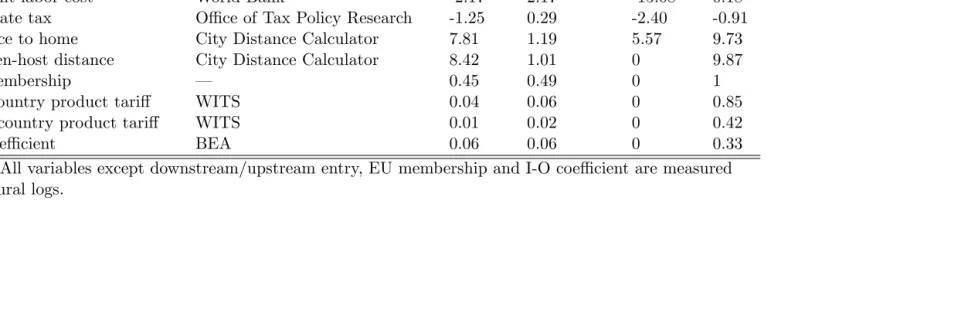
Table A.1: Summary statistics
Variables Source Mean Std. dev. Min Max
downstream entry AMADEUS 0.007 0.08 0 1
upstream entry AMADEUS 0.002 0.04 0 1
GDP WDI 26.24 1.35 23.85 30.00
real unit labor cost World Bank -2.17 2.17 -15.08 0.18
corporate tax O¢ce of Tax Policy Research -1.25 0.29 -2.40 -0.91
distance to home City Distance Calculator 7.81 1.19 5.57 9.73
between-host distance City Distance Calculator 8.42 1.01 0 9.87
EU membership — 0.45 0.49 0 1
host-country product tari¤ WITS 0.04 0.06 0 0.85
home-country product tari¤ WITS 0.01 0.02 0 0.42
I-O coe¢cient BEA 0.06 0.06 0 0.33
Note: All variables except downstream/upstream entry, EU membership and I-O coe¢cient are measured in natural logs.
Figure 1: Renault’s global production network (the darker and lighter areas represent upstream and downstream production locations, respectively)
[image:31.612.143.470.427.630.2]0 0.02 0.04 0.06 0.08 0.1 0.12 0.14 0.16
1 10 100
Number of invested countries
D
ens
ity 2007
[image:32.612.160.458.112.308.2]2005
Figure 3: The distribution of French MNCs by the number of invested countries
0
1
2
3
4
5
fr
eq
ue
nc
y
(%
)
0 5000 10000 15000 20000
distance
[image:32.612.145.473.402.638.2]0
.00
0
05
.0
001
.00
0
15
d
ens
ity
0 5000 10000 15000 20000
distance
[image:33.612.143.471.89.330.2]downstream subsidiaries vertically linked subsidiaries
Figure 5: The kernel density of between-subsidiary distance: downstream subsidiaries v.s. ver-tically linked subsidiaries
0
10
20
30
fr
eq
ue
nc
y
(%
)
0 .2 .4 .6 .8 1
tariff
[image:33.612.143.472.411.649.2]0
2
4
6
8
d
ens
ity
0 .2 .4 .6 .8
tariff
[image:34.612.144.470.255.492.2]downstream subsidiaries vertically linked subsidiaries