Munich Personal RePEc Archive
Equal Strength or Dominant Teams:
Policy Analysis of NFL
Biner, Burhan
University of Minnesota, Department of Economics
25 March 2009
Equal Strength or Dominant Teams:
Policy Analysis of NFL
Burhan Biner ∗†
University of Minnesota JOB MARKET PAPER
March 2, 2009
Abstract
In North America, professional sports leagues operate mostly as cartels. They employ certain policies such as revenue sharing, salary caps to ensure that teams get high revenues and players get high wages. There are two major hypotheses regarding the talent distribution among the teams that would maximize the total revenues, dominant teams rule and equal strength team rule. This paper examines the revenue structure of National Football League and proposes policy recommendations regarding talent distribution among the teams. By us-ing a unique, rich data set on game day stadium attendance and TV ratus-ings I am able to measure the total demand as a function of involved teams talent levels. Reduced form regres-sion results indicates that TV viewers are more interested in close games, on the other hand stadium attendees are more interested in home teams dominance. In order to identify the true effects of possible policy experiments, I estimate the parameters of the demand for TV as functions of team talent , fixed team and market variables by using partial linear model described as in Yatchew (1998) which uses non-parametric and difference-based estimators. I then estimate the demand for stadium attendance using random coefficients model by using normative priors for the 32 cities that hosts the teams. Estimated demand for TV ratings and stadium attendance corroborates the findings of reduced form regressions, stadium demand and TV demand working against each other. We therefore propose a somewhat equal strength team policy where big market teams has a slight advantage over the others. Total revenues of the league is maximized under such a policy.
Keywords: Perfect Competition, Dominant Team, Cartels.
JEL Classifications: C14, C34, L52, L83
∗I would like to thank Ryan Rebholz of Pro Football Hall of Fame for helping me find the crucial TV data. I also
wish to thank Tom Holmes, Kyoo il Kim, Erzo Luttmer, Turkmen Goksel for their helpful discussions with me. I would also like thank Olivia Hansburg for lending me her expertise in data. Lastly I am grateful to the Economics Department of the University of Minnesota for financial support. All errors are my own.
†Department of Economics, University of Minnesota, 1035 Heller Hall, 271-19th Avenue South, Minneapolis, MN,
1
Introduction
Professional sports leagues in North America are good examples of cartels. Most of them have some
sort of exemption status from the laws of commerce that the rest of the economy has to abide by.
They have a league governing body formed by the owners and players that plan and take care of
the problems of the league. The league generates revenue through games and the revenue is shared
between team owners and players. They are mostly free to adopt policies on governing the league
as they wish. The league primarily wants to increase the total revenue made throughout the league
in order to increase the salaries for players and profits for team owners. There are various actions
available to the league including imposing a salary cap or revenue sharing.
There are two major hypotheses regarding how leagues use relative strength of teams to increase
total revenues, player salaries and fan utility. The first is to follow the dominant teams rule. Pick
a few teams that have revenue making advantage over the others and make sure that they have a
stronger team ensuring that their fans will generate higher revenue. MLB, to some extent follows
this, New York Yankees, Boston Red Sox, New York Mets and Chicago Cubs have clear advantage
in revenue generation over the other teams. The second hypothesis is to distribute talent among
the teams ”evenly”, ensuring a high level of competition and thereby attracting higher demand for
the game.
In this paper we are going to empirically assess the superiority of these two hypotheses over
each other for National Football League.
Among all professional sports leagues National Football League is by far the most lucrative
sports league. In 2007, the NFLs annual revenues exceeded $7 billion. In contrast, Major League
Baseball generated revenues of just over $6 billion. Basketball and hockey lag far behind. The
National Basketball Associations annual revenues stand at $3.3 billion. Bringing up the rear among
the Big Four team sports leagues, the National Hockey Leagues revenues reach $2 billion annually1.
There are clearly certain things going right with NFL. Popularity of the game has been increasing
every passing year along with its’ revenue making potential. Clearly their policies are working
for the league. They have been employing a salary cap rule along with revenue sharing due to a
collective bargaining with NFL Players Association.
1
This paper argues that in NFL, TV audience in general likes to watch somewhat close games
while fans attending the games like to see their teams dominate the other team. On average 66-70
percent of a team’s revenue comes from media deals. Since most of the revenue comes from the
media it’s best to have a policy that advocates a somewhat equal team strength.
There is a rich literature in sports economics. Most of the literature is in theoretical sports
economics with a few empirical research papers mainly done in simple regressions. In the first
mathematical model of a professional sports league, El-Hodiri and Quirk,(1971), examine whether
the current organization of professional team sports will lead to equalization of playing strengths.
They develop a dynamic model involving wages, revenues, trades, the draft, skill level, and the
probability of winning a game. Profit maximization is not consistent with the equalization of
playing strengths unless all teams are affected equally by a change in strength of one team in terms
of gate receipts, or if the home team receives at least half of the gate receipts and all teams have
the same revenue function. Additionally, to ensure equalization, there must be a constant supply of
new playing skill and no cash sales. Equal strengths will converge regardless of the initial allocation
of talent. Fewer teams and a quicker depreciation of talent will speed up the convergence process.
Atkinson, Stanley, and Tschirhart (1988), develop a model of a professional sports league which
shows how revenue sharing encourages an optimal distribution of resources among teams. The
league tries to devise an incentive scheme that will induce agents to maximize total output. The
agents, on the other hand, receive private non-monetary benefits which are not shared. This leads
to classical principal agent problem. Empirically, they show that that revenue sharing has desirable
properties for the NFL, but is partially mitigated if teams are not profit maximizers.
Fort and Quirk, (1995), develop a profit maximizing model of a professional sports league.
They discuss the issues in determining the definition of winning, whether it be season-long winning
percentage or championship prospect. The effects of the reserve system versus free agency are
examined. A salary cap results in equal playing strengths and would be adopted if the cap is
sufficiently low. They argue that it is the only incentive mechanism which can maintain league
viability and competitive balance.
Empirical papers in Sports Economics are mostly done with very limited data. This is usually
due to lack of team level game day data. Most of the empirical analysis is done for aggregate level
level data on consumers. The big elephant in the room is unobserved heterogeneity that’s hard to
touch due to lack of data at the individual level. Specifically it’s hard to measure the ”fanness” of
consumers. In European sports leagues people are more attached to their teams, in some cases cult
like cultures exist. This is not really the case in US. However, we still see that type of behavior for
certain teams. Detroit Lions have been a losing team for quite some time, yet they manage to sell
almost capacity for most of their games. Whether this is due to fans’ connection to their teams or
some other reason is hard to guess.
Welki and Zlatoper, (1991), analyzes the game day stadium attendance in NFL for 1991 season.
In their paper they analyze the attendance in terms of ticket price, home team record, visiting team
record, income level of home team population, temperature and some other dummy variables. Their
Tobit analysis finds a clear bias for home team record which supports our hypothesis for game day
attendance. However, their data is only for one season which raises doubts about the validity of
the results. In their (1999) paper they analyze the games for 1986 and 1987 seasons. In that paper
they use betting lines to measure how close a game is expected to be by the general audience. They
find that fans do care about closeness of games and quality of the playing teams, especially home
team.
Carney and Fenn,(2004), on the other hand analyzes the TV ratings for NFL games in 2000
and 2001 seasons. In their analysis they find that closeness of the games matter by using winning
records of opposing teams. They use various variables such as player race, coach race. However
their analysis relies on local TV ratings which is a relatively minor consideration for the general
discussion since most of the revenue comes from national media deals.
There is no research done on NFL for the entire revenue scheme. Our analysis is done for both
TV ratings and stadium attendance making it possible for us to come up with a better policy
analysis. TV ratings data we use is national level data and game day attendance data is a very rich
panel data that spans 14 years.
The rest of the paper proceeds as follows. Section 2 introduces the theoretical model. Section 3
introduces the data used in the paper. In Section 4, we use reduced form regressions and random
coefficient models for both sets of data to estimate demand and discusses the results. Section 5
2
Theory
This section first presents a simple theoretical model for sports demand both in terms of stadium
attendance and TV ratings. Then I discuss some analytical results.
In general the audience cares about a game’s potential characteristics such as how close the
game will be, likelihood of their team winning the game, the week the game is played and other
variables. We can represent the first two characteristics in terms of the talent levels of the teams.
Let t1 be the home team’s talent level and t2 be the visiting team’s talent level. Probability of
home team winning has to be positively correlated with home team’s talent level. Without loss of
generality assume that
W in1,2 =
t1
t1+t2
α
(1)
where 0 < α < 1. This assures us that probability of winning is an increasing and concave
function of t1. Probability of winning for the visiting team is defined similarly
Closeness of the game has to be correlated with the talent difference of the teams. Without loss
of generality assume that
Close1,2 =|t1−t2|β (2)
where −1< β≤0.
The TV ratings for a particular game will be the product of winning probability and closeness.
Similarly, stadium attendance will be a product of winning probability and closeness. Here, αis the
elasticity of demand with respect to winning probability, β is the elasticity of demand with respect
to closeness.
We assume that there are two types of cities, big cities and small cities. In an environment like
this it’s normal to assume that team types are also correlated with the city types. Teams in big
cities should be able to bring more demand and more revenue. Therefore I am going to assume
that big city teams will have t1 talent and small city teams havet2 talent. This model is equivalent
to the model where there is one big city team and one small city team facing each other certain
face each other ω1 times at the big city team’s turf, ω2 times at the small city team’s turf. We can
assume that ω1+ω2 = 1, moreover we will normalize the total talent to 1,t1+t2 = 1. Even though
total talent used by the league can be less than 1 we will assume that it will be binding. In other
words, everyone in the talent pool will be employed.2 Let the size of the big city ben
1 and the size
of the small city be n2.
Under these assumptions total demand for stadium attendance will be
Att=n1ω1
t1
t1+t2
α1
t2
t1+t2
α2
|t1−t2|β 1
+n2ω2
t1
t1+t2
α3
t2
t1+t2
α4
|t1 −t2|β 2
(3)
We are assuming that elasticities of winning probabilities and closeness are different for each
city. On the other hand TV ratings will be
Rating =n1ω1
t1
t1+t2
α5
t2
t1+t2
α6
|t1−t2|β 3
+n2ω2
t1
t1+t2
α7
t2
t1+t2
α8
|t1−t2|β 4
(4)
Since we are only looking national level TV data, for ratings can assume that elasticities of
winning and closeness are same throughout the league. We have no way of seeing which city
watched which game. Total demand for the game will be the sum of Att and Rating.
Proposition 2.1 Total demand is maximized whent1 =t2 if βi = 06 for at least one i= 1,2,3,4.
Proof See appendix.
Clearly the degree of how much people care about close games is important. If they don’t care
at all, rather they care about their team winning then maximum demand is achieved depending on
the relative elasticity of winning probabilities, relative size of the cities and ratio of the type of big
cities and small cities.
Corollary 2.2 If TV viewers care more about close games and stadium attendees care more about
their home team winning then total demand is maximized when t1 =t2.
2
Proof This is a simple application of Proposition 2.1.
3
Data
3.1
TV Data
Since almost 70 percent of operating income of every team under the current revenue sharing rule
comes from media deals, it’s only fitting to first analyze TV ratings. Our TV ratings data comes
from Football Hall of Fame archives. Data spans nationally televised games for 1972-1978, 1981 and
1983. Data includes preseason games, regular games and playoff games. Almost all of the preseason
games have ratings available, however there are no betting lines quoted for them. Not all of the
regular games have been nationally televised. Monday night, Thursday, Friday and Saturday games
are usually nationally televised. On Sundays, usually one or two games are picked and televised
by national stations. Even though there is 1943 games in this period we have only 491 games with
ratings.
In order to analyze the effect of close games on TV ratings we have collected Las Vegas Betting
lines data for the corresponding games using Washington Post archives. Lines are quoted as one
single number representing which team is favored by how many points. It represents public’s
perception of an upcoming game. It’s a good candidate for measuring how close a game will be
if it’s measured around zero. If betting line between Vikings playing at Green Bay is reported
as -5, this means Green Bay is favored by 5 points. The more the betting lines negative, the
more home team is favored. If betting lines are quoted as positive that means visiting team is
favored. Clearly a betting line close to zero means that game is perceived to be tight. Bookies who
publish betting lines usually have their own formulas. In order to do a consistent estimation, it’s
important to find consistent betting lines. This is especially important since I use betting lines for
different periods, 1970’s and 1994-2007 period. Our comparison shows that they are following the
same line. Bookies in general use win ratios, streaks of teams involved in the upcoming game in
their formulas. Correlation between visiting team win ratio and betting lines for the TV data is
about 0.47, correlation between home team win ratio and betting lines is about -0.46 which is a
are 0.38 and -0.38 respectively. They also use game specific information such as the place of the
game, weather conditions during the game3 and team specific information such as injuries. I will
denote these information as Σ. Therefore, betting line between team i and team j at time t can be
formulated as
Betijt =E[P ointi,t−P ointj,t|W inrati,t−1, W inratj,t−1, Streaki,t−1, Streakj,t−1,Σ] (5)
Here P ointi,t and P ointj,t are the number of points team i and team j will score at the game
respectively.
Summary of the data is given in Table 1 in the appendix.
A single national ratings point represents one percent of the total number of television
house-holds. Since they are normalized with respect to the number of households with TV for that year
it’s a good measure for the TV demand for the game. There is quite a bit variation in the rating
data to explain. The lowest rating we have is recorded on a game that coincided with a World
series game. The highest was recorded on a Super Bowl game. Standard error for playoff games
is about 7.6, standard error for regular games is 3.8. Viswinper and Homwinper are winning
percentages of visiting and home teams prior to every game respectively. Betting lines only measure
how close a game is expected to be, in other words they measure the relative perceived strength
of the opposing teams, they do not measure individual qualities of the teams. We use winning
percentages for this purpose. Win-loss streaks of opposing teams going into each game measures
the order of wins. Order of wins are clearly important for our analysis as well since win percentages
are not a good measure of how teams are doing going into a specific game. After four games, if
a team has two wins and two losses clearly when those games are won make a difference. If they
won the last two games, they go into next games on a winning spree and usually audience respond
positively to that. If they win on an alternating schedule then the effect of the last win is not as
much. Homebase measures the possible population who would be interested in watching home
team’s game, visbase is similarly defined. It’s calculated by using team’s division city populations
. The rest of the variables are dummy variables describing the game day. Worldseries corresponds
to the games coincides with MLB playoff games, Doubleheader corresponds to games that are
3
televised consecutively on the same day. On the other hand, weekcount measures the week the
game is played, as the season progresses we see increased attention towards the game. Since betting
lines show winning bias, we also include the absolute value of the betting lines, we only care how
close a game is perceived to be not who is likely to win, absline measures this. By using absolute
value of betting lines we introduce nonlinearity into our estimation, however at the same time we
lose the directional information that betting lines bring into the table.
3.2
Stadium Data
Our stadium data covers the games between 1994-2007. I collected attendance data for every
regular game using various web sites. I then collected betting lines corresponding to these games
from Mrnfl.com. Mrnfl.com reports the betting lines published on Washington Post, therefore it
matches the betting lines I used for TV ratings. Summary of the data is given in Table 2 in the
appendix.
Some of the variables here are same as what I used for TV ratings. I include stadium size,
stadium cost adjusted for 1938 prices, stadium age, attendance normalized by stadium size, MSA
population, MSA income per capita, difference between attendance and stadium size, average season
price adjusted for 1994 prices. Unfortunately at the panel level some of these variables are useless.
Price is seasonal therefore has no effect on game by game estimation, stcost on the other hand is
constant and in the usual reduced regression it has negative coefficient. Dif measures the difference
between attendance and stadium size, difratis the normalized difference ratio. I have to use difrat
for censored regression model. Stadium size here is not a hard upper bound for attendance. It’s
most of the time adhered but in some cases some teams can add a few more seats to their stadiums.
This is especially true for warm climate teams such as Tampa Bay. Nevertheless, the stadium sizes
listed on team web sites are mostly observed, there are only 382 cases out of 3448 games that
4
Estimation
4.1
TV Demand
The most important aspect of our TV Data is that we observe that games expected to be close bring
higher ratings. Our hypothesis is that TV audience has a different utility function than the typical
fan. In terms of the model we introduced, elasticity of winning probability for TV audience is very
close to zero. Instead of going through the hassles of driving, waiting for the queues, bathrooms,
parking, dealing with the rowdy fans they’d like to sit at the comfort of their house and watch a nice
game. Average game watcher on TV is mostly interested in games that are competitive rather than
his team definitely winning. Let (t1, t2) be the talent level of both of the teams. Utility function
of TV audience has to be a decreasing function of |t1 −t2|, increasing function of win records of
both teams. Utility maximization of TV audience problem gives us a plausible demand function.
It simply leads to the following assumption for TV ratings: I assume that the TV ratings is a
production of betting lines , home team’s win percentage, visiting team’s win percentage and other
market and game specific variables. This is along the lines of the theory I introduced in Section 2.
In order to account for the negative values that win-loss streaks and betting lines take I will use
the following log-linear modeling:
Ratingijt =A∗eα∗abslineijt ∗eβ∗homwinpert ∗eγ∗viswinpert ∗eΩ (6)
where Ω ={homestreak, visstreak, homebase, visbase, totbase, dummyvariables}andidenotes
the home team,j denotes visiting team. We do expect the coefficient forabsline to be negative and
coefficients of win percentages of both teams to be positive of close magnitude when we log-linearize
the production function for ratings. In the log-linear model ln(y) = β1+β2x, one-unit increase in
x leads to 100×β2% change in y.
One of the problems with the estimation of TV ratings is that our data has sample selection
issues. Scheduling of most of the games are done before the season starts. Monday night games are
scheduled this way just as Thanksgiving day games at Detroit and Dallas. Regular Sunday games
and some Saturday games on the other hand are selected by the broadcast company a week prior
as well but they are in general quite competitive and fit the selection criteria. In order to correct
for selection I use the heckman probit model. Selection equation is determined by Homewinper,
Viswinper, Homestreak, Visstreak. In order to use heckman selection model I need exclusion
restriction variables. Betting lines are determined to some extent using these variables but the
correlation is not that much. Especially, correlation between betting lines and win-loss streaks are
very low. We use the type II Tobit model:
y1 = x1β1+u1 (7)
y2 = 1[xδ2+v2>0] (8)
The second equation is the selection equation. y2 and xare always observed,y1 is observed only
when y2 = 1. We have observations for Homewinper, Viswinper, Homestreak, Visstreak
on every game. The fact that win-loss streak can be negative and we look at games where teams
are more likely to be in equal strengths ensure that y2 can be 0. For those games we don’t have
any ratings. With further assumptions that (u1, v2) is independent of x with zero mean, v2 ∼
Normal(0,1) and E(u1|v2) = γ1v2 we can estimate this model. A little bit manipulation gives us
the following:
E(y1|x, y2 = 1) =x1β1+γ1λ(xδ2) (9)
where λ is the inverse Mills ratio. We can estimate this model using the Heckitprocedure:
We first obtain the probit estimate ˆδ2 from the model
P(yi2 = 1|xi) = Φ(xiδ2) (10)
using all observations. Then, obtain the estimated inverse Mills ratios ˆλi2 =λ(xiδˆ2). Then, we
obtain ˆβ1 and ˆγ1 from OLS regression on the selected sample, yi1 on xi1, ˆλi2.
A simple t-test of the estimate of the inverse Mills ratio λ is a valid test for sample-selection
bias.
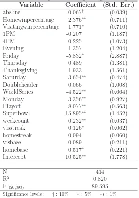
Results are corroborating our hypothesis. TV audience cares more about how close the games are.
Clearly the negative coefficient on the absolute value of betting lines show that people care more
about close games, it’s statistically significant at the level of 10%. For every one unit difference in
team talent ratings decrease by 6.7 percent. This is a significant effect on the ratings. Home team’s
winning percentage is favored a little more than the visiting team winning percentage. Even when
corrected for selection we see that closeness of the games are significantly important.
Linear regression unfortunately gives us only a general idea about how the audience is reacting
to games on TV. It averages out quite a bit of information and doesn’t use the nonlinearity. If we
look at Figure 1-3, we see that ratings are very nonlinear in terms of betting lines, win percentages.
In order to account for nonlinearity in the model I use two other specifications to model the TV
demand. The other specification for TV Ratings as a function of explanatory variables I use is
LogRatingijt =α+β∗abslineγijt+τ homwinper η
ijt+ψviswinperijtκ +... (11)
The other variables are in linear form. Nonlinear estimation of this specification is reported in
Table 7. Even when accounted for nonlinearity we see that absline has negative coefficient albeit
it’s statistical significance is not much. The power of absline,γ, comes out 1.655. This supports
the linear regression model we estimated earlier. The coefficients and powers of win ratios are quite
significant and again supports our results from linear regression.
Throughout all these models one other common result we see is that population base of a team
is also very important. In other words teams that play in big cities or big markets tend to draw
more audience to TV, this is of course expected but as a possible policy we can see that big market
teams should have better teams in order to maximize the revenues. This is especially true for home
teams that has a large audience. It’s better to televise games that’s played on a big city team turf.
The last specification I use is the semiparametric regression formulated by Yatchew:
yijt =f(zijt) +xijtβ+ǫijt (12)
where z is a random variable, x is a p-dimensional random variable. E[y|x, z] =f(z) +xβ and
ǫijtis iid mean-zero error term such thatV ar[y|x, z] =σǫ2. The functionf is a smooth, single valued
(f(z)) parts are additively separable.
We follow the methodology suggested by Yatchew (1997). We first estimate the nonparametric
nonlinear part by locally weighted least squares method as described in Yatchew (2003). Then we
do the linear least squares on yi =π+xβ where π is the estimate from lowess method.
We assume that E(ǫ|x, z) = 0 and that V ar(ǫ|x, z) = σ2
ǫ, z’s have bounded support and have
been rearranged so that they are in increasing order. Suppose that the conditional mean of x is a
smooth function of z, say E(x|z) = g(z) where g′ is bounded and V ar(x|z) = σ2
u. Then we may
rewrite x=g(z) +u. Differencing yields
yi−yi−1 = (xi−xi−1)β+ (f(zi)−f(zi−1)) +ǫi−ǫi−1
= (g(zi)−g(zi−1))β+ (ui−ui−1)β+ (f(zi)−f(zi−1)) +ǫi−ǫi−1
∼
= (ui−ui−1)β+ǫi −ǫi−1
Thus, the direct effect f(z) of the nonparametric variable z and the indirect effect g(z) that
occurs through x are removed. Suppose we apply the OLS estimator of β to the differenced data,
that is,
ˆ
βdif f =
P
(yi−yi−1)(xi−xi−1)
P
(xi−xi−1)2
(13)
Then, substituting the approximationsxi−xi−1 ∼=ui−ui−1andyi−yi−1 ∼= (ui−ui−1)β+ǫi−ǫi−1
into above and rearranging, we have
n1/2(ˆβdif f −β)∼= n
1/2 1
n P
(ǫi−ǫi−1)(ui−ui−1)
1
n P
(ui−ui−1)2
(14)
We can show that the above equation converges in distribution to N0,1.5σǫ2
σ2
u
. Our estimator
will be consistent.
Bottom line is, the estimation method we have here relies heavily on first differencing. After
that we take the simple OLS estimator and then use kernel regression to get the nonparametric
part. On the linear part we are using win ratios, streaks and other dummy variables. There is a
possible. Moreover, differencing here is crucial because we difference the trends out from win ratios.
For the nonlinear part I use betting lines as explanatory variable. Results are reported in Table 8.
The only difference here is that home team’s win percentage has much more significance than the
visiting team’s win percentage.
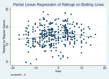
On the other hand when we use the betting lines themselves for the nonparametric part and
absolute value of betting lines in the linear part we get a much better picture. Using absolute value
of betting lines in the linear part ensures us that positive trends from previous weeks are trended
out. We can see this in Figure 1. If we don’t use absolute value of betting lines in the linear part,
for regular games we get the Figure 2. Figure 2 is a better indicator, it tells us that demand is
maximized when betting lines are close to zero. However, the curvature around zero is not as high
as in Figure 1.
0
10
20
30
Ratings
−20 −10 0 10 20
lines
bandwidth = .8
[image:15.612.364.539.316.443.2]Partial Linear Regression of Ratings on Betting Lines
Figure 1: TV Ratings against betting lines, abso-lute value of betting lines and other variables.
10
15
20
25
Ratings for Regular Games
−20 −10 0 10 20
lines
bandwidth = .8
[image:15.612.93.268.317.442.2]Partial Linear Regression of Ratings on Betting Lines
Figure 2: Regular game TV Ratings against bet-ting lines and other variables.
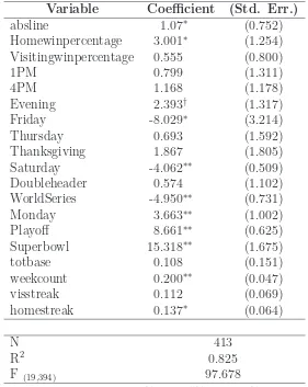
Table 8 and table 9 shows the results. When we use absline in the linear part, we are getting a
positive coefficient, this is due to the fact that most of the effect has gone onto nonparametric part
that includes betting lines. The other results are similar with table 9, home team’s win ratio is still
more important than visiting team win ratio. Home team’s population again is important.
The most important result from semiparametric estimation is that our hypothesis is supported
again. TV audience is more interested in close games.
4.2
Stadium Attendance Demand
For the stadium case I am going to report linear fixed effect estimation results along with random
linear fixed effect model, xijt includes absline, homwinrat, viswinrat, homstreak, visstreak
and other dummy variables. One of the problems with using absline as explanatory variables here
is that we lose quite a bit of information by doing that. We are losing the directional interpretation
of betting lines, in other words which team is favored. If the coefficient of absline comes up as
negative the interpretation is straightforward, fans like games that are close. If it comes up as
positive interpretation is vague, it most probably means they like blow-out games but sinceabsline
doesn’t tell us which team is favored we have to use other variables to come up with that result.
The first model is usual fixed effects panel data OLS estimation:
Attijt=α+x
′
ijtβ+ǫijt (15)
Attendance is limited by number of seats available to fans, therefore it’s important take this
censoring into account. As I pointed out in Section 3, censoring is not observed for every game.
For some games, some teams manage to post attendance more than stadium size, nevertheless this
is not a big problem since I censor any attendance over the stadium size and use the stadium size
as attendance for that particular game.
Att⋆ijt =α+x′ijtβ+ǫijt ,ǫijt ∼N(0, σi2) (16)
where Attijt=Att∗ijt if Attijt∗ < stdsizei and Attijt =stdsizei otherwise.
Clearly, fans in this case care much more about their own team’s strength since the coefficient
of home team’s winning percentage is very high compared to visiting team winning percentage.
Moreover, the coefficient on betting lines show a small bias towards home team’s relative strength
when it’s done with betting lines only rather than absolute value of the lines. As I pointed out before,
the interpretation of absolute value of betting lines is problematic, we do get that it is positive and
people care about blow out result. The fact that coefficient of homwinrat is significantly bigger
than the coefficient of viswinrat tells us that the blow out should be done by home team. If the
home team goes into game as a clear favorite, for every 1 unit advantage over the visiting team
the attendance is likely to increase by by 6 percent of the stadium size. Censored regression on
betting lines itself gives us a better interpretation. In table 12, we see that coefficient of betting
much better indicators corroborating our previous result. Stadium attendees care more about their
home team winning. We can assume that elasticity of closeness for stadium attendees is almost
zero.
If we however do the estimation team by team we see the effect of lines varying quite a bit. In
some cases such as in Arizona, fans are more interested in the visiting team rather than the home
team. When done with absolute values however we expect the coefficient to be negative, we are not
getting that but the coefficient is very close to zero. Team records are much better predictions of
the expectations of the fans.
It’s natural to think that consumers in different cities have different preferences, therefore
dif-ferent coefficients for difdif-ferent games and games in general. For example, people in New York might
care about Philadelphia games more than Arizona games.
A parsimonious model for the relationships between attendance and betting lines can be obtained
by specifying a team-specific random intercept ζ1j and a team-specific random slope ζ2j for (xij):
yij = β1 +β2xij +ζ1j+ζ2jxij +ǫij (17)
= (β1+ζ1j) + (β2+ζ2j)xij +ǫij (18)
We assume that the covariate xij is exogenous with E(ζ1j|xij) = 0, E(ζ2j|xij) = 0, and
E(ǫij|xij, ζ1j, ζ2j) = 0.
We will, as is usually done, assume that, given xij, the random intercept and random slope have
a bivariate normal distribution with zero mean and covariance matrix Σ.
Following Rossi, Allenby and McCulloch (2005), I use a hierarchical Bayesian model with a
mixture of four normal priors to account for the random coefficients. I use EM algorithm to estimate
the game day attendance. Table 13 and 14 shows the results. I then go onto show predicted Bayesian
posterior distribution for the teams.
Results are again as we predicted. Coefficient of betting lines is negative albeit very small.
However win ratio of home team again has a very high coefficient compared to win ratio of visiting
team. Figures 9-12 shows the density distribution of random coefficients we use to estimate our
attendance increase only by .00048%. On the other hand if we increase home team’s win record by
one unit (hypothetically), attendance increase by 5 percent. This clearly shows that home team’s
record is much more important for fans to attend. Home team fans would like to see their team
going dominant into a game.
5
Conclusion
The estimation results in Section 4 clearly shows that TV viewers and stadium attendees display
different type of preferences for the game. TV ratings are determined mostly by close games with
possibly strong teams playing each other. Figure 1 and 2 shows that maximum ratings are attained
when lines are close to zero. Moreover, big city teams are drawing bigger audiences to their games.
Coupled with this fact, it’s better to have as many close games and these games should be played
among teams that has larger fan base. On the other hand stadium attendance is determined by
home team’s dominance. In a city, fans are much more likely to attend a game if they think their
team is more likely to win. Therefore, it’s better to give some bias in the distribution of talent
to big city teams. Nevertheless, since most of the revenue is obtained through media deals we
suggest that talent distribution among the teams should be more towards an even distribution. It’s
imperative that there should be some bias towards teams that have bigger fan base. Of course,
this is a policy that should be adopted if there is a sensible revenue sharing policy throughout the
league. Here we are assuming that the NFL Commissioner acts as a Social Planner and has the
means to redistribute the revenue generated by this cartel. With a policy of this sort, it’s pretty
easy to increase the size of the total revenue league makes and increase the individual teams’ share.
Under this regime players on average are more likely to see their salaries go up as well since the
total revenue made will increase considerably thereby increasing team owners’ shares and players’
wages. If there is no redistribution of revenue in place then a policy that favors big city teams even
a little bit is bound to backfire in the future since small city teams will get weaker considerably in
time. Big city teams will likely use the revenues they make to attract better talent and get stronger
as time progresses. This should have adverse effects on player salaries on average even though a
few high talent players will likely see their wages go up much higher.
and Stadium attendance are covered, it’s pretty straightforward to do a policy analysis as to how
the distribution should actually be done. Actual numerical experiments can be done to simulate
the effects of any redistribution of talent. One should also observe that winning percentages are
nonlinear functions of betting lines. Therefore this makes it easier to do analysis for TV Ratings.
On the other hand, for stadium attendance since we have recovered the random coefficients the
policy analysis should be done to calculate the probability of fans attending a game depending on
the betting lines. Unfortunately we do not have yet data on player salaries and player talent. The
next step in this research will be correlating the player salaries to their talent level and coming up
with profit function for the league so as to see the effects of a possibly policy like salary cap.
References
[1] ATKINSON, SCOTT; LINDA AND TSCHIRHART, JOHN. “Revenue Sharing as an Incentive
in an Agency Problem: An Example from the National Football League”,RAND Journal of
Economics, Vol. 19, pp. 27-43, Spring 1988.
[2] CARNEY, SHANNON and FENN, AJU. “The Determinants of NFL Viewership: Evidence
from Nielsen Ratings”, Colorado College Working Paper, October 2004.
[3] EL HODIRI, MOHAMED AND QUIRK, JAMES. “An Economic Model of a Professional Sports
League”,Journal of Political Economy, Vol. 79, pp. 1302-1319, November/December 1971.
[4] FORT, RODNEY AND QUIRK, JAMES. “Cross-subsidization, Incentives, and Outcomes in
Professional Team Sports Leagues”,Journal of Economic Literature, Vol. 33, pp. 1265-1299,
September 1995.
[5] KESENNE, STEFAN. “The Impact of Salary Caps in Professional Team Sports”,Scottish
Jour-nal of Political Economy, Vol 47, pp. 422-430, 2000.
[6] ROSSI, P., ALLENBY G. AND MCCULLOCH R. “Bayesian Statistics and Marketing,” John
Wiley and Sons, 2005.
[7] SZYMANSKI, STEFAN. “The Economic Design of Sporting Contests”, Journal of Economic
[8] VROOMAN, JOHN. “A General Theory of Professional Sports Leagues”, Southern Economic
Journal, Vol. 61,4, pp 971-990.
[9] WELKI, ANDREW and ZLATOPER, THOMAS. “US Professional Football: The Demand for
Game-Day Attendance in 1991”,Managerial and Decision Economics, Vol. 15, pp. 489-495,
1994.
[10] WELKI, ANDREW and ZLATOPER, THOMAS. “US Professional Football Game-Day
At-tendance”,American Economic Journal, Vol. 27, No. 3, pp. 285-298, 1999.
[11] YATCHEW, A., “An Elementary Estimator of the Partial Linear Model”, Economic Letters,
Vol. 57: 135-43, 1997.
[12] YATCHEW, A., Semiparametric Regression for the Applied Econometrician, Cambridge
Uni-versity Press, Cambridge, UK, 2003.
A
Proofs
Proof of Proposition 2.1
If at least one of the βi 6= 0, then limt1→t2|t1 −t2|
βi = ∞, since −1 < β
i < 0. Moreover,
limt1→t2
t1
t1+t2 = 1
2. Therefore,
lim
t1→t2
t1
t1+t2
αi
|t1 −t2|βi → ∞ (19)
Since for any other combination of (αi, βi) the total profit will be finite we conclude that
max-imum is achieved when t1 =t2. In other words, whenever closeness is important it leads our total
A
Results
Table 1: Summary statistics for TV ratings
Variable Definition Mean Std. Dev. Min. Max. N
Table 2: Summary statistics for game day attendance
Variable Definition Mean Std. Dev. Min. Max. N
weekdate Week day the game played 6.494 1.554 1 7 3448
line Betting lines -2.55 5.874 -24 20 3448
week Week the game played 9.144 4.968 1 17 3448 att Attendance 64520.151 10313.258 15131 90910 3433 yearweek Year of the game 2000.668 3.994 1994 2007 3448 stdsize Stadium size 70210.216 6969.578 41203 91665 3448 viswinrat Visiting team win ratio before the game 0.502 0.262 0 1 3448 homwinrat Home team win ratio before the game 0.499 0.262 0 1 3448 monday 1 if game is played on Monday 0.068 0.252 0 1 3448 thursday 1 if game is played on Thursday 0.019 0.135 0 1 3448 friday 1 if game is played on Friday 0.009 0.093 0 1 3448 saturday 1 if game is played on Saturday 0.026 0.159 0 1 3448 sunday 1 if game is played on Sunday 0.879 0.326 0 1 3448 dif Difference between attendance and stadium size -5701.219 8804.909 -57010 14856 3433 Visteamstreak Visiting Team win-loss streak before the game 0.158 2.61 -12 15 3448 Homteamstreak Home Team win-loss streak before the game -0.125 2.656 -14 14 3448 absline Absolute value of betting lines 5.406 3.431 0 24 3448 Priceadjusted Average season ticket prices in 1994 dollars 40.622 8.679 23.93 70.48 3448 stcost Stadium cost in 1938 dollars 19647038.373 11734284.431 125000 51020166.7 3448
stdage Stadium age 19.374 13.94 0 81 3448
10
20
30
40
50
rating
−40 −20 0 20
lines
Figure 3: Ratings against betting lines for all games.
10
20
30
40
50
rating
0 .2 .4 .6 .8 1
[image:23.612.92.268.68.198.2]Hometeamwinpercentage
Figure 4: Ratings against Home Team Win Per-centages for all games.
10
20
30
40
50
rating
0 .2 .4 .6 .8 1
[image:23.612.363.539.69.198.2]Visitingteamwinpercentage
Figure 5: Ratings against Visiting Team Win Per-centages for all games.
20000
40000
60000
80000
100000
att
−20 −10 0 10 20
line
[image:23.612.366.539.408.538.2] [image:23.612.93.267.409.538.2]Table 3: Reduced regression on log ratings for all games
Variable Coefficient (Std. Err.)
absline -0.067† (0.039)
Homewinpercentage 2.376∗∗ (0.711)
Visitingwinpercentage 1.771∗ (0.710)
1PM -0.207 (1.187)
4PM 0.225 (1.073)
Evening 1.357 (1.204)
Friday -5.832∗ (2.887)
Thursday 0.489 (1.381)
Thanksgiving 1.933 (1.561)
Saturday -3.654∗∗ (0.474)
Doubleheader 0.066 (1.008)
WorldSeries -4.522∗∗ (0.664)
Monday 3.356∗∗ (0.927)
Playoff 8.077∗∗ (0.563)
Superbowl 15.895∗∗ (1.452)
weekcount 0.232∗∗ (0.037)
visstreak 0.126∗ (0.062)
homestreak 0.094 (0.060)
visbase -0.089 (0.211)
homebase 0.517∗ (0.221)
Intercept 10.525∗∗ (1.778)
N 414
R2 0.820
F (20,393) 89.595
Table 4: Reduced regressions on log ratings for playoff games
Variable Coefficient (Std. Err.)
absline -0.212 (0.179)
Homewinpercentage 8.730 (7.356)
Visitingwinpercentage 16.569∗∗ (5.972)
4PM 1.400 (0.881)
Saturday -4.402∗∗ (0.958)
Doubleheader 4.073 (2.628)
WorldSeries 0.000 (0.000)
Monday 2.957 (2.336)
Superbowl 16.069∗∗ (3.134)
weekcount 1.381∗∗ (0.343)
visstreak 0.054 (0.164)
homestreak -0.189 (0.141)
visbase -0.137 (0.686)
homebase 0.077 (0.714)
Intercept -17.003 (10.954)
N 69
R2 0.865
F (13,55) 27.21
Table 5: Reduced regressions on log ratings for regular games
Variable Coefficient (Std. Err.)
absline -0.068† (0.038)
Homewinpercentage 2.602∗∗ (0.685)
Visitingwinpercentage 1.522∗ (0.694)
1PM 0.134 (1.223)
4PM 0.718 (0.999)
Evening 0.370 (1.132)
Friday -5.341∗ (2.705)
Thursday 0.641 (1.367)
Thanksgiving 2.300 (1.552)
Saturday -2.044∗∗ (0.607)
Doubleheader -1.450 (1.117)
WorldSeries -4.540∗∗ (0.611)
Monday 3.549∗∗ (1.003)
weekcount 0.185∗∗ (0.036)
visstreak 0.092 (0.067)
homestreak 0.109 (0.067)
visbase -0.093 (0.215)
homebase 0.539∗ (0.228)
Intercept 11.698∗∗ (1.774)
N 345
R2 0.598
F (18,326) 26.956
Table 6: Heckman selection results
Variable Coefficient (Std. Err.)
Equation 1 : rating
absline -0.077∗ (0.036)
1PM -0.688 (1.164)
4PM -0.237 (1.059)
Evening 0.689 (1.181)
Friday -6.042∗ (2.749)
Thursday 0.628 (1.351)
Thanksgiving 1.805 (1.529)
Saturday -3.611∗∗ (0.468)
Doubleheader -0.048 (1.014)
WorldSeries -4.108∗∗ (0.644)
Monday 3.452∗∗ (0.928)
Playoff 8.418∗∗ (0.533)
Superbowl 15.678∗∗ (1.496)
weekcount 0.230∗∗ (0.036)
visbase -0.144 (0.206)
homebase 0.499∗ (0.214)
Intercept 17.629∗∗ (1.795)
Equation 2 : select
Homewinpercentage 0.957∗∗ (0.146)
Visitingwinpercentage 0.954∗∗ (0.150)
visstreak 0.040∗∗ (0.014)
homestreak 0.041∗∗ (0.014)
Intercept -1.825∗∗ (0.122)
N 1857
Log-likelihood -1877.62
χ2(16) 1415.189
Table 7: Nonlinear least squares regression of log ratings on the explanatory variables
Variable Coefficient (Std. Err.)
α 2.474∗∗ (0.107)
β -0.001 (0.003)
γ 1.655 (1.357)
τ 0.124∗∗ (0.042)
η 1.494 (1.038)
ψ 0.082∗ (0.042)
κ 1.300 (1.309)
visstreak 0.006† (0.004)
homestreak 0.005 (0.004)
onepm 0.018 (0.069)
fourpm 0.042 (0.063)
evening 0.083 (0.070)
friday -0.358∗ (0.168)
thursday 0.007 (0.081)
thanksgiving 0.155† (0.092)
saturday -0.169∗∗ (0.028)
doubleheader -0.032 (0.059)
worldseries -0.361∗∗ (0.039)
monday 0.185∗∗ (0.054)
playoff 0.374∗∗ (0.033)
superbowl 0.372∗∗ (0.085)
weekcount 0.013∗∗ (0.002)
totbase 0.014† (0.008)
N 414
R2 0.742
Table 8: Semiparametric Estimation of Ratings with absline as linear variable
Variable Coefficient (Std. Err.)
absline 1.07∗ (0.752)
Homewinpercentage 3.001∗ (1.254)
Visitingwinpercentage 0.555 (0.800)
1PM 0.799 (1.311)
4PM 1.168 (1.178)
Evening 2.393† (1.317)
Friday -8.029∗ (3.214)
Thursday 0.693 (1.592)
Thanksgiving 1.867 (1.805)
Saturday -4.062∗∗ (0.509)
Doubleheader 0.574 (1.102)
WorldSeries -4.950∗∗ (0.731)
Monday 3.663∗∗ (1.002)
Playoff 8.661∗∗ (0.625)
Superbowl 15.318∗∗ (1.675)
totbase 0.108 (0.151)
weekcount 0.200∗∗ (0.047)
visstreak 0.112 (0.069)
homestreak 0.137∗ (0.064)
N 413
R2 0.825
F (19,394) 97.678
Significance levels : †: 10% ∗ : 5% ∗∗: 1%
−.15
−.1
−.05
0
Normalized Attendance Difference
0 5 10 15 20 25
Absolute Value of Betting Lines
[image:29.612.164.449.113.654.2]Fitted censored regression Normalized attendance difference
Table 9: Semiparametric Estimation of Ratings of Regular games
Variable Coefficient (Std. Err.)
weekcount 0.133∗ (0.056)
Homewinpercentage 2.126∗ (0.853)
Visitingwinpercentage 1.856∗ (0.916)
1PM -2.090 (1.585)
4PM -0.025 (1.247)
Evening -0.359 (1.361)
Friday -5.129 (3.164)
Thursday 1.441 (1.633)
Thanksgiving 2.730 (1.862)
Saturday -1.676∗ (0.712)
Doubleheader -1.342 (1.274)
WorldSeries -4.686∗∗ (0.718)
Monday 3.633∗∗ (1.149)
visstreak 0.104 (0.082)
homestreak 0.084 (0.085)
homebase 0.676∗ (0.274)
visbase -0.162 (0.252)
N 344
R2 0.621
F (17,327) 31.524
Significance levels : †: 10% ∗ : 5% ∗∗: 1%
−.3
−.2
−.1
0
Normalized Attendance Difference
−20 −10 0 10 20
Betting Lines
Fitted censored regression Normalized attendance difference
[image:30.612.161.448.115.655.2]Betting Lines used for regression
Table 10: Fixed effects panel estimation for attendance ratio
Variable Coefficient (Std. Err.)
absline 0.0014∗∗ (0.0005)
week -0.002∗∗ (0.000)
homwinrat 0.049∗∗ (0.007)
viswinrat 0.002 (0.006)
visstreak 0.002∗∗ (0.001)
homstreak 0.004∗∗ (0.001)
monday 0.044∗∗ (0.007)
thursday 0.027∗ (0.012)
friday 0.005 (0.018)
saturday -0.003 (0.011)
Population 0.000∗∗ (0.000)
Income 0.000∗∗ (0.000)
Intercept 0.317∗∗ (0.028)
N 3433
R2 0.169
F (43,3389) 57.623
Significance levels : †: 10% ∗ : 5% ∗∗: 1%
0
100
200
300
400
Density
−.01 −.005 0 .005 .01
[image:31.612.360.543.503.635.2]Predicted random coefficients for lines
Figure 9: Posterior distribution for coefficients of betting lines.
0
5
10
15
20
Density
−.15 −.1 −.05 0 .05 .1
Predicted random coefficients for home win ratios
[image:31.612.88.271.503.637.2]Table 11: Random effects censored regression results on attendance ratio
Variable Coefficient (Std. Err.)
Equation 1 : difrat
absline 0.002∗∗ (0.001)
week -0.002∗∗ (0.000)
homwinrat 0.057∗∗ (0.008)
viswinrat 0.002 (0.007)
visstreak 0.003∗∗ (0.001)
homstreak 0.004∗∗ (0.001)
monday 0.049∗∗ (0.008)
thursday 0.033∗ (0.015)
friday -0.015 (0.021)
saturday -0.008 (0.012)
Intercept -0.096∗∗ (0.014)
Equation 2 : sigma u
Intercept 0.068∗∗ (0.009)
Equation 3 : sigma e
Intercept 0.110∗∗ (0.001)
N 3433
Log-likelihood 1952.545
χ2
(10) 206.555
Significance levels : †: 10% ∗ : 5% ∗∗: 1%
0
20
40
60
80
Density
−.02 0 .02 .04 .06
Predicted random coefficients for visiting team win ratios
Figure 11: Posterior distribution for coefficients of visiting team winning ratios.
0
5
10
15
Density
−.3 −.2 −.1 0 .1
[image:32.612.359.544.512.649.2]Predicted random coefficients for Intercept
Table 12: Censored regression on betting lines
Variable Coefficient (Std. Err.)
Equation 1 : difrat
line -0.00006 (0.0003)
homwinrat 0.059∗∗ (0.008)
viswinrat 0.002 (0.007)
week -0.002∗∗ (0.000)
visstreak 0.002∗∗ (0.001)
homestreak 0.005∗∗ (0.001)
monday 0.049∗∗ (0.008)
thursday 0.032∗ (0.015)
saturday -0.008 (0.012)
friday -0.015 (0.021)
Intercept -0.088∗∗ (0.014)
Equation 2 : sigma u
Intercept 0.068∗∗ (0.009)
Equation 3 : sigma e
Intercept 0.110∗∗ (0.001)
N 3433
Log-likelihood 1948.085
χ2(10) 197.237
Significance levels : †: 10% ∗ : 5% ∗∗: 1%
Table 13: Random Coefficients Model with absolute value of betting lines
Variable Coefficient (Std. Err.)
Equation 1 : attratio
absline 0.002∗ (0.001)
homwinrat 0.060∗∗ (0.007)
viswinrat 0.004 (0.007)
Intercept 0.880∗∗ (0.013)
N 3433
Log-likelihood 2863.799
χ2
(3) 81.549
[image:33.612.189.427.531.696.2]Table 14: Random coefficient estimation with betting lines
Variable Coefficient (Std. Err.)
Equation 1 : attratio
line -0.000048 (0.001)
homwinrat 0.051∗∗ (0.013)
viswinrat 0.005 (0.008)
visstreak 0.002∗∗ (0.001)
homstreak 0.004∗∗ (0.001)
week -0.002∗∗ (0.000)
monday 0.041∗∗ (0.007)
thursday 0.027∗ (0.013)
saturday -0.008 (0.011)
friday -0.012 (0.018)
Intercept 0.905∗∗ (0.015)
N 3433
Log-likelihood 2918.139
χ2(10) 137.599