3D Nonlinear XFEM Simulation of Delamination in Unidirectional Composite Laminates: A Sensitivity Analysis of Modeling Parameters

3D Nonlinear XFEM Simulation of Delamination in

Unidirectional Composite Laminates: A Sensitivity

Analysis of Modeling Parameters

Damoon Motamedi, Abbas S. Milani*

School of Engineering, University of British Columbia, Kelowna, Canada. Email: *_{[email protected]}

Received August 9th_{, 2013; revised September 9}th_{, 2013; accepted September 20}th_{, 2013}

Copyright © 2013 Damoon Motamedi, Abbas S. Milani. This is an open access article distributed under the Creative Commons At- tribution License, which permits unrestricted use, distribution, and reproduction in any medium, provided the original work is prop- erly cited.

ABSTRACT

This article presents a three-dimensional extended finite element (XFEM) approach for numerical simulation of de- lamination in unidirectional composites under fracture mode I. A cohesive zone model in front of the crack tip is used to include interface material nonlinearities. To avoid instability during simulations, a critical cohesive zone length is de- fined such that user-defined XFEM elements are only activated along the crack tip inside this zone. To demonstrate the accuracy of the new approach, XFEM results are compared to a set of benchmark experimental data from the literature as well as conventional FEM, mesh free, and interface element approaches. To evaluate the effect of modeling parame- ters, a set of sensitivity analyses have also been performed on the penalty stiffness factor, critical cohesive zone length, and mesh size. It has been discussed how the same model can be used for other fracture modes when both opening and contact mechanisms are active.

Keywords: Composite Materials; Fracture Properties; Double Cantilever Beam; Extended Finite Element; Cohesive Zone Model

1. Introduction

Today, composite structures are widely used in high tech engineering applications including aeronautical, marine and automotive industries. They have high strength-to- weight ratios, good corrosion resistance, and superior fracture toughness. In addition, they can be engineered based on required strength or performance objectives in each given design. Although fiber-reinforced composites have been proven to provide numerous advantages, they are still prone to cracking, interlaminar delamination, fiber breakage and fiber pull-out failure modes. Among these, delamination is known to be the most common mode that often occurs because of a weak bonding be-tween composite layers, an existing crack in the matrix, broken fibres, fatigue or severe impact.

For modeling delamination, numerous investigations have been performed over the past few decades. Hiller- borg et al. [1] introduced a combination of the finite ele- ment method (FEM) and an analytical solution to simu-

late crack growth. The approach is frequently referred to as “fictitious crack modeling” where a traction-separa- tion law instead of a conventional stress-strain relation- ship is utilized in the crack tip zone to capture degrada- tion of material properties due to the damage. Xu and Needleman [2] applied an energy potential function to implement a cohesive zone model (CZM) concept during the analysis of interface debonding. Further investiga- tions on improving cohesive interface models were per- formed in [3-9]. Based on these reports, CZM has been proven to be capable of modeling “large process zones”— in the present case the composite delamination interface. When utilized in the simulation of progressive delamina- tion, however, some disadvantages of large process zone approach have been noted. These include numerical in- stability (e.g., elastic snap-back), reduction of stress in- tensity upon the delamination initiation, and the soften- ing of the original body in the process zone [10].

In other investigations, a relatively new feature of FEM, known as the extended finite element method (XFEM), has been implemented for numerical modeling

of discontinuities. The original XFEM approach was introduced by Belytschko and Black [11] and enhanced by Moёs et al. [12]. They implemented the concept of the partition of unity method (PUM), which was earlier em- ployed to develop a method for modeling discontinuity in materials [13]. In the basic XFEM, a modified Heaviside step function is implemented to model the crack surface by adding extra degrees of freedom to each node of the so-called “enriched elements” [12]. Further improve- ments of XFEM were presented in different applications with plastic/elastic material domains, fluid/solid phases,

and static/dynamic loadings [14-21]. Moёs and Belyts-

chko [22] introduced an analysis framework capable of considering cohesive cracks and frictional contact be- tween crack surfaces in two-dimensional (2D) problems. Later on, a similar approach was implemented to model cohesive cracks in concrete specimens [23]. The applica- tion of the 2D model was also extended to composite materials in [24], by means of utilizing XFEM including CZM with a linear traction-separation law to predict de- lamination.

In the present article, the above cohesive crack model- ing approach is applied to 3D domains and used for pre- dicting mode I fracture behaviour of unidirectional lami- nates. To this end, an ABAQUS user-element subroutine has been developed to model the nonlinear behaviour of composite samples (T300/977-2 carbon fiber reinforced epoxy and AS4/PEEK carbon fiber reinforced polyether ether ketone) under the standard double cantilever beam (DCB) test. Cohesive zone was added to enrich elements in the crack front under a bilinear traction-separation law. In addition, a technique is introduced for simple imple- mentation of the cohesive zone by avoiding material sof- tening due to the application of large process zone. Name- ly, to decrease the computational time and to avoid insta- bility during simulations, a critical length of cohesive zone in vicinity of the crack tip is defined such that the user-defined XFEM elements are only assigned inside this region. It is shown that the new technique avoids predefining a complete delamination path along the spe- cimen length, and leads to more realistic prediction of experimental data. Finally, a set of sensitivity analyses have been performed to identify effects of different mod- eling parameters, while comparing the results to conven- tional FEM, the mesh free method, and the interface element approaches.

2. Nonlinear Extended Finite Element

(XFEM): A Review of Fundamentals

There are several numerical techniques available for ana- lyzing stress and displacement fields in engineering struc-

tures, including FEM, finite difference method (FDM) and meshless methods. Among these, FEM has shown popularity in terms of modeling material nonlinearity effects as well as different complex geometries and boundary conditions. As addressed earlier, the FEM ca- pability in modeling discontinuities was first realized by introducing the partition of unity [13] into the approxi- mating functions—later known as the extended finite element [11,22]. In some complex crack problems, XFEM has demonstrated more accurate and stable solutions while the conventional finite element results were rough or highly oscillatory [22].

In XFEM, as an advantage, the finite element mesh is generated regardless of the location of discontinuities. Subsequently, search algorithms such as the level-set or fast marching methods can be utilized to identify the lo- cation of any discontinuity with respect to the existing mesh, and also to distinguish between different types of required enrichments for affected elements. Finally, addi- tional auxiliary degrees of freedom are added to the con- ventional FEM approximation functions in the selected nodes around the discontinuity. To review the method mathematically, let us assume a discontinuity (a crack) within an arbitrary finite element mesh, as depicted in

Figure 1.

The displacement field of a point x, _ug

 

 

 

   

f

I _J

g

I I J J

I J

n N n N

u x  x u  x  x a

 

 





 

  is the conventional shape function, 

 

enrichment function, N is the finite element mesh nodes

and _Nf _{is the number of enriched nodes of the mesh,}

I

u is the classic degrees of freedom at each node and

J

a are the additional enriched degrees of freedom at the

Jth _{node. The displacement approximation in Equation (1)}

can be implemented in numerical solutions of Linear Elastic Fracture Mechanics (LEFM) to predict displace- ment fields. Considering the total potential energy gov- erning the problem, one can write:

d _fb _ud _ft _ud

   

          







where  , , u, _fb _{and f}t _{are the stress tensor,} strain tensor, displacement vector, body forces and trac- tion forces, respectively.  is the traction boundary and

 is the integration domain. Discretizing Equation (2)

and applying the variational formulation, the following matrix-form equation is obtained:

where U denotes a vector containing the nodal parame-

ters including ordinary degrees of freedom “u_{” and the}

enriched degrees of freedom “a”:

 

,

U  u a (4)

The stiffness matrix K and the external load vector F are defined as:

uu ua ij ij e

ij au aa

ij ij K K K K K       

  (5)





,

u a

i i i

F  F F (6)

The stiffness components rs





ij

K r s u a in Equa-

tion (5) include the classical (uu_{), enriched (}aa_{) and cou-}

pled (ua_{) arrays of XFEM approximation:}

 





d , ,

rs r s

ij i j

K 

_

where C _{is the material constitutive relationship arrays} and Bi is the shape functions derivatives matrix defined for each degree of freedom in 3D problems as:

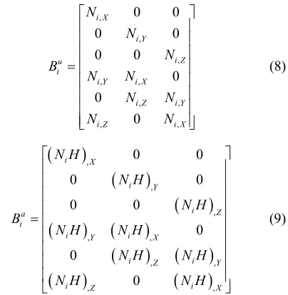
, , , , , , , , , 0 0 0 0 0 0 0 0 0 i X i Y i Z u i

i Y i X

i Z i Y

i Z i X

N N N B N N N N N N                      (8)





































i Y i X

i Z i Y

i Z i X

N H

N H

N H B

N H N H

N H N H

N H N H

                       (9)

Ni is the conventional FEM shape functions, H is the

Heaviside step function value; X, Y and Z are the refer- ence coordinates. For numerical implementation, integra- tion points can be included by the following shifting

amendment in a

i

B [22]:

crack

Enriched by Heaviside function

Influence domain of node J

J

Figure 1. The influence domain of node J in an arbitrary finite element mesh.

 

 





 

 





 

 





 

 







 

 



 

 







 

 



 

 







 

 



i i _X

i i _Y

i i _Z

a i

i i _Y i i _X

i i _Z i i _Y

i i _Z i i _X

N H H

N H H

N H H

B

N H H N H H

N H H N H H

N H H N H H

where i is the numerical integration (e.g., Gauss quad- rature) coordinates in the local system. In order to in- clude cohesive properties to XFEM formulations, Khoei

et al. [25] introduced an approach based on contact mod-

eling (to be discussed further in Section 3). Their approach also considered a 3D modeling of nonlinear (large deforma- tion) formulation by forming a total tangential matrix based on both material and geometrical stiffness matrices:

T ep _d T _d

T Mat Geo S S

K K K B D B G M G

 

  

_

_

, ep, ,

S S

B D G M are the strain gradient matrix, the ma-

terial constitutive matrix, Cartesian gradient matrix and

re-arranged second Piola-Kirchhoff stress matrix, Sij,

using the identity matrix, I_{3 3} , defined as: (see Equa- tions (12)-(16); including the footnotes).

0 0 0 0 0 0 0 0 0 0 0 0 0 0 0 0 0 0 i i i i u i i i i i i N X N X N X N Y N G Y N Y N Z N Z N Z    _        _        _  _       _         _       _           _        _    (14)





































3 3 3 3 3 3 3 3 3 3 3 3

.

XX XY XZ

S YY YZ

ZZ

S I S I S I

M S I S I

sym S I

                 (16)

In Equations (12) to (16), x, y and z represent the spa- tial material coordinate system and also the Heaviside function value is interpolated at each integration point.

3. Cohesive Interface Modeling

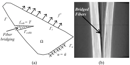
Before In composite materials when the crack propaga- tion initiates, a damage zone appears in front of the crack tip and dissipates the high stress intensity expected in LEFM. This damage zone can be interpreted as a cohe- sive zone (e.g., due to fiber bridging) which complicates the identification of crack tip (Figure 2). In the presence

i i i

i i i

i i i

u i

i i i i i i

i i i i i i

N x N y N z

X X X X X X

N x N y N z

Y Y Y Y Y Y

N x N y N z

Z Z Z Z Z Z

B

N x N x N y N y N z N z

Y X X Y Y X X Y Y X X Y

N x N x N y N y N z N z

Z Y Y Z Z Y Y Z Z Y Y Z

                                       _    _    _                _    _    _              N_i x N_i x N_i y N_i y N_i z N_i z

Z X X Z Z X X Z Z X X Z

Гu

f t

Гcohh

fcoh = T

u = ū Гt Ω Г Fiber bridging Bridged Fibers

(a) (b)

Figure 2. (a) A general body in the state of equilibrium un- der different tractions and boundary conditions; (b) Exam- ple of fiber bridging from an actual tested sample under fracture mode I.

of a cohesive crack, the total potential energy formula- tion can be rewritten to consider the traction forces over the crack surface. Neglecting body forces, the related governing equation is written as:

t t

d d d

coh coh

f u T v

   

          







where _ft_{, T}t _{and vare the external forces on domain} boundary, cohesive traction vector on the crack surface and the crack tip opening displacement vector, respec- tively. Based on constitutive behaviour of the interface material, the traction forces are directly related to the opening and sliding displacements of the crack faces. A

transformation matrix

 

rearrange the displacement nodal vector and rewrite the crack opening displacement and cohesive traction as fol- lows [23].

Coh

v B u (18)

Interface Coh

T D B u (19)

where DInterface represents the interface material proper- ties matrix.

Conventionally, in order to add traction forces into

XFEM, a “contact” bond region within enriched ele- ments is assumed and the gauss integration points within this bond are considered for formulation of the contact stiffness matrix. Applying the same idea for the cohesive traction, a non-zero thickness cohesive zone model can be established in the form of tangential stiffness matrix for 3D problems [25]:

 

T T

T

d d

d T Mat Geo Coh

ep

S S

Coh Interface Coh

K K K K

B D B G M G

B D B

           







3.1. Choosing an Interface Traction-Separation Law

Needleman [26] implemented a potential function to model cohesive zone behaviour for ductile interfaces as follows.





0 0 0

, 1 1 n exp n exp t

n t

n n t

v v v

v v

v v v

         

      

  (21)

where φ0, vn, vt, vn0, vt0 are the material fracture energy,

normal and tangential crack opening displacements, normal and tangential model parameters, respectively. This potential function has been utilized in many re- search works to extract the mechanical behavior of inter- face layers; however it has shown some disadvantages such as introducing softening and numerical instability to FEM, especially during crack propagation steps [10]. Also, it neglects the material behavior dependency on different fracture modes which can result in a non-con- servative estimation of critical forces. To overcome the aforementioned problems, a rigid cohesive model was proposed in [27]. In this model, a high initial stiffness is applied to the interface elements and the degradation of













































































i i i

i i i

i i i

a i

i i i i i i

i i i i

N H x N H y N H z

X X X X X X

N H x N H y N H z

Y Y Y Y Y Y

N H x N H y N H z

Z Z Z Z Z Z

B

N H x N H x N H y N H y N H z N H z

Y X X Y Y X X Y Y X X Y

N H x N H x N H y N H y

Z Y Y Z Z Y Y Z

                                                                                  

































i i i i i i

N H z N H z

Z Y Y Z

N H x N H x N H y N H y N H z N H z

Z X X Z Z X X Z Z X X Z

material is assessed by damage indices to reduce the pen- alty stiffness, KPen, continuously. Despite reliable results acquired by this approach, numerical instabilities were observed when the material degradation was commenced in front of the cracked region and the convergence be- came dependent of the penalty stiffness. In the present

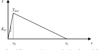
work, a bilinear traction-separation law (Figure 3) was

implemented to model the interface material degradation in the opening mode in both normal and tangential direc- tions, which has been also widely used in earlier investi- gations [4,28-30]:

















0

0

elastic part

1 softening part

0 decohesion part

Pen

Pen f

f

T K v v v

T D K v v v v

T v v

  

 _{   }



  



(22)

T is the interfacial strength of the material and D is the damage index defined as:

0 0

f

f

v v v

D

v v v

 _ 

 _ _



  (23)

Remark:For modeling contact/closing modes, a simi-

lar approach is used to consider a diagonal matrix for Interface

D where a penalty stiffness value is assigned to

each diagonal component depending on the normal or tangential (sliding) behaviour of the interface [25]. For general-purpose fracture simulations, our model through a user-defined code in ABAQUS recognizes whether the crack faces are in the opening or closing mode and ap- plies the corresponding DInterface for each enriched ele- ment.

In the cohesive opening mode all the three diagonal

terms of DInterface may be considered identical and the

model assumes the element degradation begins when the crack relative displacement exceeds the critical crack tip opening value, v0. In turn, v0 can be defined in terms of

the penalty stiffness, KPen, and the maximum interfacial

strength, Tmax, as follows.

max 0

Pen T v

K

 (24)

Therefore, selecting an appropriate value of KPen be-

comes critical to establish a stable cohesive finite ele-

ment model. While choosing a large value of KPen may

help true estimation of the elements stiffness before the crack initiation, it will reduce the required critical rela- tive displacement value for the crack initiation and, hence, cause numerical instability upon the crack initia- tion, known as the elastic-snap back. Using a reasonable value for KPen can lead to accurate results while attaining a low computational cost. Earlier works have been un-

dertaken to formulate KPen based on different types of

Tmax

T

v

v0 vf

Kpe

Figure 3. A bilinear traction-separation law for modeling the interface material degradation.

material properties. Turon et al. [10] proposed a simple

relationship between the transverse modulus of elasticity, Etran, the specimen thickness, t, and the penalty stiffness, KPen:

tran Pen

E K

t 

 (25)

whereα was proposed to be equal to 50 to prevent the

stiffness loss. Nonetheless, in several other cases, a com- parison between numerical analysis and experimental results is required to identify an optimum value of pen- alty stiffness.

3.2. Length of the Cohesive Zone

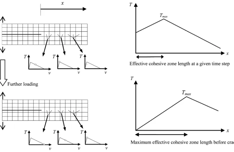
Another important factor in the numerical simulation of delamination is the length of cohesive zone. As opening or sliding displacement increases, elements in the cohe- sive zone gradually reach the maximum interfacial strength and the maximum stress rises up to the critical interfacial stress ahead of the crack tip. Upon this point, the affected elements’ stiffness moves into the softening region of traction-separation law and experiences an ir- reversible degradation. The maximum length of cohesive zone occurs when the crack tip elements are considered

debonded completely (Figure 4), and then the simulation

should move to the next stage by expanding the crack length. The criterion for such complete opening is dis- cussed in the subsequent sub-section. Considering a cor- rect value of the length of cohesive zone is essential in numerical modeling of delamination, to prevent difficul- ties due to implementing the traction-separation law in- stead of a conventional (continuous) constitutive rela- tionship. Other researchers have studied extensively this

topic for general crack problems. Hillerborg et al. [1]

proposed a characteristic length parameter for isotropic materials as follows.

2 max

C cz

G

l E

T

 (26)

Figure 4. Formation steps of the cohesive zone in front of crack tip during numerical simulation.

the material, respectively. Other equations can be found for estimating the cohesive zone length [10]. For various traction-separation laws, Planas and Elices [31] intro- duced a different equation for isotropic materials. For

orthotropic materials, like composite laminates, Yang et

al. [32] discussed the possible effects of longitudinal,

transverse and shear moduli as well as the laminate thick-

ness, t, on the cohesive zone length. Subsequently, they

suggested a modified formulation for measuring the co- hesive zone length in slender composite laminates:

1 4 3 4 2

max

C cz tran

G

l E t

T

 

  

  (27)

For FEM implementations, the number of elements at- taining a cohesive constitutive behavior is directly related to the cohesive zone length. Accordingly, a range of val- ues for proper mesh size in cohesive zone has been pro- posed by other researchers [33] and [34], yet it is deemed difficult to estimate an exact value that can be optimum for all fracture simulations.

3.3. Crack Initiation and Growth Criteria

In conventional application of cohesive zone models, a predefined crack path is utilized to model the cracking behavior in the structure using a separate layer of cohe- sive elements.

The crack evolution (opening and propagation) can only occur by failure of these elements under a given loading condition and failure criteria. Damage indices are normally employed to reduce the affected elements’

stiffness in subsequent simulation steps. In the present work, however, a separate set of cohesive elements have not been employed; instead, by applying the level-set method, nonlinear XFEM elements are embedded with a cohesive behavior in front of the crack. This in turn re- duces the cost of computations and prevents the trac- tion-separation law from imposing unnecessary softening into simulations, especially at the stage of crack evolu- tion. As a threshold criterion, the crack growth is directly related to the energy release rate utilizing the J-integral method [35]:

1

1

d j

k j ij j

u

J W n

x

 





 

 _  _ 



 



where Г is an “arbitrary” contour surrounding the crack-

tip with no intersection to other discontinuities, W is the strain energy density defined as W = (1/2)σijεij for a lin- ear-elastic material, nj is the jth _{component of the outward}

unit normal to Г, δ1j is Kronecker delta, and the coordi- nates are taken to be the local crack-tip coordinates with the x1-axis parallel to the crack face. Equation (28) may

not be in a well-suited form for finite element implemen- tations; hence an equivalent form of this equation has been proposed by exploiting the divergence theorem and additional assumptions for homogeneous materials [36]:

, d

j

k ij k

k V

u

J W q V

x  



 

  _  

 



where the integral paths  and c denote near-field

tion region (hatched region in Figure 5) which is sur- rounded by _. _ and _c; V_ represents the near- field domain of crack-tip where in LEFM stress singular- ity is expected (Figure 5). q is a function varying linearly from 1 (near the crack-tip) to 0 (towards the exterior

boundary, ). To extract the energy release rate from

the J-integral, the crack-axis components of the J-inte- gral is required to be evaluated by the following coordi- nate transformation:

 

0

l lk k

J   J (30)

where αlk is the coordinate transformation tensor and θ0 is

the crack angle with respect to the global coordinate sys-

tem. The tangential component of the J-integral corre-

sponds to the rate of change in potential energy per unit crack extension, namely, the energy release rate G:

0

1cos 0 2sin 0

l

GJ J  J  (31)

In Mode I and Mode II fracture analyses, the crack propagation occurs when the measured energy release rate exceeds its critical value. This can also be depicted in the mixed-mode crack propagation where the failure prior to the complete debonding is evaluated by the fol- lowing power law [37]:

1

I II III

IC IIC IIIC

G G G

G G G

  

     

   

     

      (32)

where GI, GIIand GIII are the energy release rates for Mode I, Mode II and Mode III; GIC, GIIC and GIIIC are the critical energy release rates for Mode I, Mode II and Mode III which can be found from standard fracture tests; α, β and γ are empirical fracture critical surface parame- ters fitted using experimental data.

If crack propagation happens in any step of the nu- merical analysis, the crack tip extends by the length of cohesive zone (e.g., Equation (27)) and presents elements debonding in the simulation. It is also expected that the energy release rate per crack extension reaches its critical value when each element in the cohesive zone exceeds the critical opening displacement, v0.

4. Illustrative Example: Numerical

Simulation of DCB Test

Double Cantilever Beam (DCB) is a standard test used to evaluate the mode I fracture toughness and failure prop- erties of materials. The DCB samples are normally fab- ricated based on ASTM D5528-01. Composite materials considered in the current study are T300/977-2 carbon fiber reinforced epoxy and AS4/PEEK carbon fiber-re- inforced polyether ether ketone which are used, e.g., in the aerospace industries to manufacture airframe struc- tures with reduced weight (instead of steel components).

VГ

x1

Гε Г

Гc

Vε

Θ0

X2

X1

x2

Figure 5. Local crack-tip co-ordinates and the contour Γ

and its interior area, VΓ.

The T300/977-2 specimens have a 150 mm length, 20 mm width, and 1.98 mm thickness for each arm, with an

initial crack length of 54 mm as shown in Figure 6. For

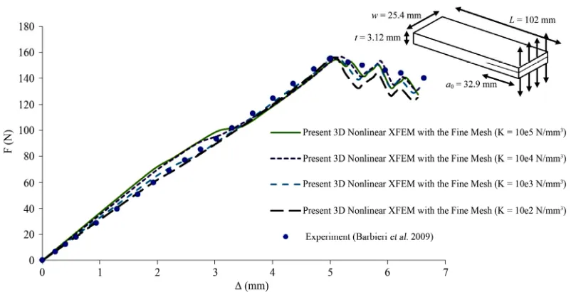
AS4/PEEK samples, specimens were 105 mm long, 25.4 mm wide and 1.56 mm thick for each arm, with a 33 mm initial crack. Material properties of each specimen are summarized in Table 1.

Previous numerical works on both types of these com- posites have been performed using cohesive interface layers via conventional finite elements and the mesh-free methods [4,10,30]. In the present study, ABAQUS finite element package was employed to implement the new 3D nonlinear XFEM approach (Sections 2 and 3) along with the CZM properties via a user-defined element sub- routine, UEL (accessible free-of-charge for research pur- poses via contacting the corresponding author). A MAT-LAB code was also developed and linked to the FEM package to undertake the analysis framework by per- forming post-processing of numerical results and evalu- ating the stability of the crack propagation as well as updating ABAQUS input files and elements properties for each step of the analysis. Results of the XFEM are also compared to other standard numerical approaches to provide further understanding of the XFEM performance in terms of the prediction accuracy and numerical stabil- ity. Next, effects of different important modeling vari- ables such as interface stiffness (the penalty factor) and the cohesive region length are studied.

4.1. Effects of Different Modeling Approaches

Turon et al. [10] investigated the effective cohesive zone length for T300/977-2 specimens. They suggested a co- hesive zone length of 0.9 mm from numerical simula-

tions on a very fine mesh (with element length, le, of

0.125 mm). Based on their work, the size of elements in the cohesive zone region should not exceed 0.5 mm and a minimum of two elements is required in this region for

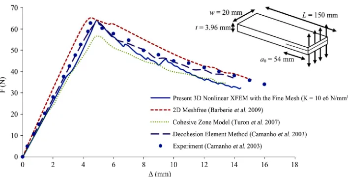
acceptable modeling results. In Figure 6, the present

Figure 6. The comparison between the global load-displacement (F-Δ) results using different analysis methods on T300/977-2 sample; For XFEM, fine mesh along with the penalty stiffness of 1 × 106 N/mm3 _{and the cohesive zone length of 1.5 mm were}

used.

Table 1. Material properties of the test samples [4,10,30] used in numerical simulations.

T300/977-2 AS4/PEEK

Elastic Properties _Properties Fracture Elastic Properties _PropertiesFracture

E11 = 150 GPa Tmax = 45 MPa E11 = 122.7 GPa Tmax = 80 MPa

E22 = E33 = 11 GPa GIC = 268 J/m2E22 = E33 = 10.1 GPa GIC = 969 J/m2

G12 = G13 = 6 GPa G12 = G13 = 5.5 GPa

G23 = 3 GPa G23 = 2.2 GPa

v12 = v13 = 0.25 v12 = v13 = 0.25

v23 = 0.5 v23 = 0.48

alty stiffness of 1 × 106 _N/mm3 _{and the cohesive zone}

length of 1.5 mm are compared to the results available in the literature by means of different types of numerical approaches [4,10] and [30].

Figure 6 shows that all the models predict a similar trend of the global load-displacement during delamina- tion. The mesh-free method [30] overestimates the stiff- ness of the material and leads to a higher peak opening force by 5%, while cohesive finite element approach [10] underestimates the resisting force by 10% in comparison to the experimental data [4]. The XFEM estimates the peak opening force by 3% difference from the experi- ment, and similar to [4] provides more conservative es- timation of the fracture behavior of the DCB samples.

4.2. Effects of Mesh Size and Cohesive Zone Length

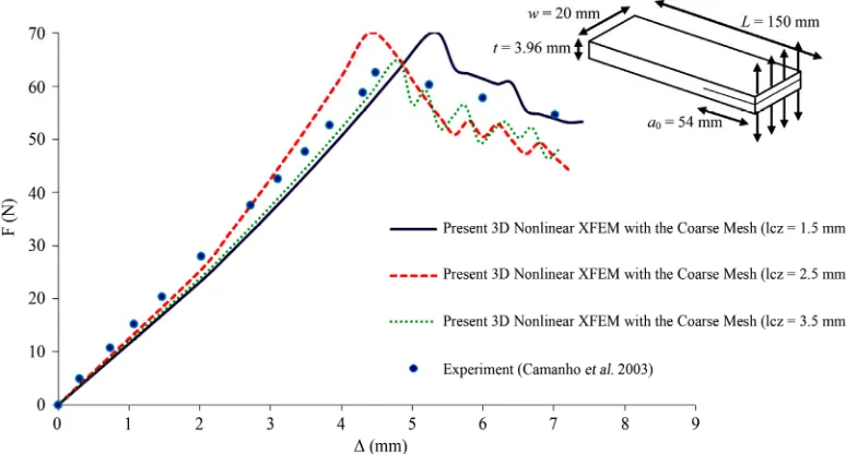
The DCB test of T300/977-2 specimens was simulated using two different mesh sizes, namely the element

lengths of 0.4 mm and 1.25 mm, to demonstrate the ef- fect of coarse and fine meshes on the XFEM results. In addition, in each case to present the influence of cohesive

zone length, simulations were rerun (Figures 7 and 8)

with different lcz values and with a fixed penalty stiffness of 1 × 106 _N/mm3 _{following [10]. Recalling Figure 7, in}

the fine mesh (le = 0.4 mm) models, it is observed that

using 3 (lcz = 1.5 mm) to 6 (lcz = 2.5 mm) elements within the cohesive zone would lead to an accurate estimation of the experimental data, while increasing this critical value to 8 (lcz = 3.5 mm) elements would introduce an unrealis- tic global softening behavior to the model which regards the previous investigation in term of mesh sensitivity [38]. In the coarse mesh (le = 1.25 mm) runs (Figure 8),

only for the case with 3 (lcz = 3.5 mm) elements, the

Figure 7. Load-displacement curve for fine mesh (le = 0.4 mm) simulation with different cohesive zone lengths for T300/977-2

sample.

Figure 8. Load-displacement curve for coarse mesh (le = 1.25 mm) simulation with different cohesive zone length for T300/

977-2 sample.

cillations to a certain degree without adapting a damping ratio to the model. This feature can be especially benefi- cial regarding computational time in explicit finite ele- ment analysis.

4.3. Effect of Different Penalty Stiffness Factors

As discussed in Section 3.1, accuracy of the bilinear trac- tion-separation law in modeling the process zone can directly depend on the penalty stiffness value, the opti- mum value of which may change from one crack prob- lem to another. In this section, in order to evaluate the accuracy of XFEM predictions against different penalty stiffness values, a set of simulations with fine mesh were

performed with a wide range of values varying from 102

N/mm3 _{to 10}5 _N/mm3_{, and with an identical cohesive}

zone length of lcz = 2.5 mm. Results are shown in Fig-

ures9 and 10 and compared to experimental data [4] for

both T300/977-2 and AS4/PEEK specimens, respectively. The XFEM results were less sensitive to the larger order of penalty stiffness values (from 103 _{to 10}5 _N/mm3_{) in}

comparison to the conventional finite element method results [10]. Finally, within the latter recommended

Pen

K range, two sets of complimentary simulations on

Figure 9. The comparison of load-displacement curves of T300/977-2 sample using different penalty stiffness values.

Figure 10. The comparison of load-displacement curves of AS4/PEEK sample using different penalty stiffness values.

ness, and vice versa. As AS4/PEEK has a higher critical energy release rate in comparison to T300/977-2 samples (Table 1), a larger cohesive zone region should be ex- pected and, hence, the sensitivity of simulations to the element size is reduced. Conversely, the crack simulation of a material with low fracture toughness would necessi- tate a smaller cohesive zone length and subsequently, would show more sensitivity to the mesh size.

5. Conclusions

The present work demonstrated the effectiveness of a combined XFEM-cohesive zone model (CZM) approach in 3D numerical simulation of Mode I fracture (delami- nation) in fiber reinforced composites in the presence of

Figure 11. The comparison between XFEM load-displacement curves for fine mesh analysis of AS4/PEEK and previous works.

Figure 12. The comparison between XFEM load-displacement curves for coarse mesh analysis of AS4/PEEK and previous works.

separation law improves the convergence of numerical simulations and reduces the mesh size sensitivity; how- ever, using conventional FEM this can again cause a sof- tening problem and reduce the peak opening force pre- diction. The XFEM approach with embedded CZM is found to be less sensitive to the aforementioned effects, particularly when the penalty stiffness value is chosen arbitrarily within the range of transverse and longitudinal moduli of the composite.

Although the present work relied on deterministic fracture behavior of the material, there is no question that in practice mechanical properties of the same composite can vary from one sample/manufacturing process to an- other, and hence “stochastic” XFEM modeling of com- posites is worthwhile [39].

6. Acknowledgements

Financial support from the Natural Sciences and Engi- neering Research Council (NSERC) of Canada is greatly acknowledged. Authors are also grateful to their col- leagues Drs. M. Bureau, D. Boucher, and F. Thibault from the Industrial Materials Institute-National Research Council Canada for their useful feedback and discus- sions.

REFERENCES

773-781.

[2] X. P. Xu and A. Needleman, “Numerical Simulations of Fast Crack Growth in Brittle Solids,” Journal of the Me- chanics and Physics of Solids, Vol. 42, No. 9, 1994, pp. 1397-1434.

[3] G. T. Camacho and M. Ortiz, “Computational Modelling of Impact Damage in Brittle Materials,” International Journal of Solids and Structures, Vol. 33, No. 20-22, 1996, pp. 2899-2938.

[4] P. P. Camanho, C. G. Dávila and M. F. De Moura, “Nu- merical Simulation of Mixed-Mode Progressive Delami-nation in Composite Materials,” Journal of Composite Materials, Vol. 37, No. 16, 2003, pp. 1415-1424.

[5] B. R. K. Blackman, H. Hadavinia, A. J. Kinloch and J. G. Williams, “The Use of a Cohesive Zone Model to Study the Fracture of Fiber Composites and Adhesively-Bonded Joints,” International Journal of Fracture, Vol. 119, No. 1, 2003, pp. 25-46.

[6] Y. F. Gao and A. F. Bower, “A Simple Technique for Avoiding Convergence Problems in Finite Element Simu- lations of Crack Nucleation and Growth on Cohesive In- terfaces,” Modelling and Simulation in Materials Science and Engineering, Vol. 12, No. 3, 2004, pp. 453-463.

[7] T. M. J. Segurado and C. T. J. Llorca, “A New Three- Dimensional Interface Finite Element to Simulate Frac- ture in Composites,” International Journal of Solids and Structures, Vol. 41, No. 11-12, 2004, pp. 2977-2993.

[8] Q. Yang and B. Cox, “Cohesive Models for Damage Evo- lution in Laminated Composites,” International Journal of Fracture, Vol. 133, No. 2, 2005, pp. 107-137.

[9] M. Nishikawa, T. Okabe and N. Takeda, “Numerical Si- mulation of Interlaminar Damage Propagation in CFRP Cross-Ply Laminates Under Transverse Loading,” Inter- national Journal of Solids and Structures, Vol. 44, No. 10, 2007, pp. 3101-3113.

[10] A. Turon, C. G. Dávila, P. P. Camanho and J. Costa, “An Engineering Solution for Mesh Size Effects in the Simu- lation of Delamination Using Cohesive Zone Models,”

Engineering Fracture Mechanics, Vol. 74, No. 10, 2007, pp. 1665-1682.

[11] T. Belytschko and T. Black, “Elastic Crack Growth in Finite Elements with Minimal Remeshing,” International Journal for Numerical Methods in Engineering, Vol. 45, No. 5, 1999, pp. 601-620.

[12] N. Moёs, J. Dolbow and T. Belytschko, “A Finite Ele- ment Method for Crack Growth without Remeshing,” In- ternational Journal for Numerical Methods in

Engineer-ing, Vol. 46, No. 1, 1999, pp. 131-150.

[13] J. M. Melenk and I. Babuška, “The Partition of Unity Finite Element Method: Basic Theory and Applications,”

Computer Methods in Applied Mechanics and Engineer- ing, Vol. 139, No. 1-4, 1996, pp. 289-314.

[14] N. Sukumar, N. Moёs, B. Moran and T. Belytschko, “Ex-

tended Finite Element Method for Three-Dimensional Crack Modeling,” International Journal for Numerical Methods in Engineering, Vol. 48, No. 11, 2000, pp. 1549- 1570.

[15] J. Dolbow, N. Moёs and T. Belytschko, “An Extended Finite Element Method for Modeling Crack Growth with Frictional Contact,” Computer Methods in Applied Me- chanics and Engineering, Vol. 190, No. 51-52, 2001, pp. 6825-6846.

[16] T. Belytschko, H. Chen, J. Xu and G. Zi, “Dynamic

Crack Propagation Based on Loss of Hyperbolicity and a New Discontinuous Enrichment,” International Journal for Numerical Methods in Engineering, Vol. 58, No. 12, 2003, pp. 1873- [17] T. Belytschko and H. Chen, “Singular Enrichment Finite

Element Method for Elastodynamic Crack Propagation,”

International Journal of Computational Methods, Vol. 1, No. 1, 2004, pp. 1-15.

[18] P. M. A. Areias and T. Belytschko, “Analysis of Three- Dimensional Crack Initiation and Propagation Using the Extended Finite Element Method,” International Journal for Numerical Methods in Engineering, Vol. 63, No. 1, 2005, pp. 760-788. [19] A. Asadpoure, S. Mohammadi and A. Vafai, “Crack Ana-

lysis in Orthotropic Media Using the Extended Finite Element Method,” Thin-Walled Structures, Vol. 44, No. 9, 2006, pp. 1031-1038.

[20] D. Motamedi and S. Mohammadi, “Dynamic Analysis of Fixed Cracks in Composites by the Extended Finite Ele- ment Method,” Engineering Fracture Mechanics, Vol. 77, No. 17, 2010, pp. 3373-3393.

[21] D. Motamedi and S. Mohammadi, “Dynamic Crack Pro-

pagation Analysis of Orthotropic Media by the Extended Finite Element Method,” International Journal of Frac- ture, Vol. 161, No. 1, 2010, pp. 21-39.

[22] N. Moёs and T. Belytschko, “Extended Finite Element Method for Cohesive Crack Growth,” Engineering Frac- ture Mechanics, Vol. 69, No. 1, 2002, pp. 813-833. [23] J. F. Unger, S. Eckardt and C. Könke, “Modelling of Co-

Applied Mechanics and Engineering, Vol. 196, No. 41-44, 2007, pp. 4087-4100.

[24] E. Benvenuti, “A Regularized XFEM Framework for Em- bedded Cohesive Interfaces,” Computer Methods in Ap- plied Mechanics and Engineering, Vol. 197, No. 1, 2008, pp. 4367-4378.

[25] A. R. Khoei, S. O. R. Biabanaki and M. Anahid, “A La- grangian Extended Finite Element Method in Modeling Large Plasticity Deformations and Contact Problems,”

International Journal of Mechanical Sciences, Vol. 51, No. 5, 2009, pp. 384-401.

[26] A. Needleman, “A Continuum Model for Void Nuclea- tion by Inclusion Debonding,” Journal of Applied Me- chanics, Vol. 54, No. 3, 1987, pp. 525-531.

[27] H. Yuan, G. Lin and A. Cornec, “Applications of Cohe- sive Zone Model for Assessment of Ductile Fracture Processes,” Journal of Engineering Materials and Tech- nology, Vol. 118, No. 1, 1996, pp. 192-200.

[28] P. Harper and S. R. Hallett, “Cohesive Zone Length in Numerical Simulations of Composite Delamination,” En- gineering Fracture Mechanics, Vol. 75, No. 16, 2008, pp. 4774-4792.

[29] C. Fan, J. P. Y. Ben and J. J. R. Cheng, “Cohesive Zone with Continuum Damage Properties for Simulation of Delamination Development in Fiber Composites and Fail- ure of Adhesive Joints,” Engineering Fracture Mechanics, Vol. 75, No. 13, 2008, pp. 3866-3880.

[30] E. Barbieri and M. Meo, “A Meshfree Penalty-Based Approach to Delamination in Composites,” Composites Science and Technology, Vol. 69, No. 13, 2009, pp. 2169- 2177.

[31] J. Planas and M. Elices, “Nonlinear Fracture of Cohesive Materials,” International Journal of Fracture, Vol. 51,

No. 2, 1991, pp. 139-157.

[32] Q. D. Yang, B. N. Cox, R. K. Nalla and R. O. Ritchie, “Fracture Length Scales in Human Cortical Bone: The Necessity of Nonlinear Fracture Models,” Biomater, Vol. 27, No. 9, 2006, pp. 2095-2113.

[33] P. P. Camanho and C. G. Dávila, “Mixed-Mode Decohe-

sion Finite Elements for the Simulation of Delamination in Composite Materials,” NASA/TM, No. 211737, 2002. [34] A. Carpinteri, P. Cornetti, F. Barpi and S. Valente, “Co-

hesive Crack Model Description of Ductile to Brittle Size-Scale Transition: Dimensional Analysis vs. Renor- malization Group Theory,” Engineering Fracture Me- chanics, Vol. 70, No. 14, 2003, pp. 1809-1839.

[35] J. R. Rice, “A Path Independent Integral and the Ap-

proximate Analysis of Strain Concentration by Notches and Cracks,” Journal of Applied Mechanics, Vol. 35, No. 1, 1968, pp. 379-386.

[36] J. H. Kim and G. H. Paulino, “The Interaction Integral for Fracture of Orthotropic Functionally Graded Materials: Evaluation of Stress Intensity Factors,” International Jour- nal of Solids and Structures, Vol. 40, No. 15, 2003, pp. 3967-4001.

[37] E. M. Wu and R. C. Reuter Jr., “Crack Extension in Fi-

berglass Reinforced Plastics,” University of Illinois, Cham- paign, 1965.

[38] M. L. Falk, A. Needleman and J. R. Rice, “A Critical Evaluation of Cohesive Zone Models of Dynamic Frac- ture,” Journal de Physique IV, Vol. 11, No. 5, 2001, pp. 543-550.