The choice between bus and light rail transit: a stylised cost benefit analysis model

Munich Personal RePEc Archive

The choice between bus and light rail

transit: a stylised cost-benefit analysis

model

Grimaldi, Raffaele and Laurino, Antonio and Beria, Paolo

DiAP Politecnico di Milano, DiAP Politecnico di Milano, DiAP

-Politecnico di Milano

2010

Online at

https://mpra.ub.uni-muenchen.de/24872/

THE CHOICE BETWEEN BUS AND LIGHT RAIL

TRANSIT: A STYLISED COST-BENEFIT ANALYSIS

MODEL

Raffaele Grimaldi1, Antonio Laurino2, Paolo Beria3

Abstract

In the last 20 years light rail and tramway schemes have been introduced in many European cities. The effects of these schemes over public transport patronage, and the benefits they have generated, seem to have sometimes been overestimated. The availability of some experiences helps in deriving some reflections about the circumstances in which light rail schemes can be truly convenient compared to bus systems.

This paper tries to give a contribution by developing a simplified model to support the choice between keeping a bus corridor or upgrading towards a light rail system. The choice is analysed on the basis of a parametrical socio-economic cost-benefit analysis. All the parameters introduced and used for a numerical simulation are discussed and some typical values from the literature are given. On the basis of these values, some feasibility abaci are drawn.

Keywords: cost-benefit analysis; bus; tram; light rail; transit; public transport.

1.

Introduction

The definition of “light rail” covers a quite wide range of solutions (NAO, 2004), from modern versions of traditional electric street tramways to automatic systems (like the Docklands Light Rail in London) or tram-train systems (like the ones present in Karlsruhe, Kassel and Saarbrücken in Germany or in RijnGouweLijn in the Nederlands). According to The

1

Corresponding author: Raffaele Grimaldi. Address: DiAP - Politecnico di Milano, Via Bonardi 3, 20133 Milano (Italy). Tel.: (+39)02.2399.5424. E-mail:

raffaele.grimaldi@polimi.it

2

Antonio Laurino. Address: DiAP - Politecnico di Milano, Via Bonardi 3, 20133 Milano (Italy). Tel.: (+39)02.2399.5424. E-mail: antonio.laurino@polimi.it

3

Paolo Beria. Address: DiAP - Politecnico di Milano, Via Bonardi 3, 20133 Milano (Italy).

International Association of Public Transport (UITP), light rail is defined

as “a tracked, electrically driven local means of transport, which can be developed step by step from a modern tramway to a means of transport running in tunnels or above ground level”. In general, the terms tramway,

light rail and light rapid transit, are used interchangeably (SDG, 2005), despite the broad variety of technical solutions.

In the last 20 years light rail and tramway schemes have been introduced in many European cities. The effects of these schemes over public transport patronage, and the benefits they have generated, seem however to have been sometimes overestimated.

The availability of some experiences helps in deriving some reflections about the circumstances in which light rail schemes can be truly convenient. This paper tries to shed a light in defining such circumstances.

We build a comprehensive formula of Net Present Value under a socio-economic cost-benefit analysis approach. We use this formula to draw some synthetic abaci that represents the thresholds of economic viability for such systems, according to some fixed parameters. The cost-benefit model is based on some simplifying hypotheses on the line structure, that however represents in our opinion a very common situation. The approach is very similar to the one used by de Rus and Nash (2007) and by de Rus and Nombela (2007) to evaluate profitability of high speed train lines. However, the problem we face is considerably much more complicated by the presence of many more significant variables (for example the regularity or the frequency of services) that can be correctly ignored in a high speed investment. The consequence of these different levels of complexity is that our three-dimensions abaci need more parameters to be fixed. This operation is done by suggesting such parameters from literature, or leaving

the “users” of this methodology to input their own specific parameters into

2.

Light rail: why and where?

In recent years, Light Rail systems (hereafter “LR”) and Bus Rapid Transit systems (hereafter “BRT”) are experiencing a renewed interest as

an attractive urban alternative to classic bus systems.

Some recent successful examples of Bus Rapid Transit applications are present in Curitiba (Pinehiro, 2005), Bogotà (Nair and Kumar, 2005), Ottawa and Brisbane (Rathwell and Schijns 2002) and in many other cities, especially outside Europe.

Broader are the experiences on LR and on the comparison with standard bus schemes.

There are different reasons that can explain public interest for LR applications. The common rationale used to justify LR is that this modality allows to meet diverse set of goals that range from economic to social and environmental considerations. The main advantages of LR with respect to bus can be summarized as follow:

higher capacity for both vehicles and line; lower operating costs;

lower noise;

smaller loading gauge (essential in city centre); more comfortable ride;

higher speed, reliability and efficiency.

On the other side, one must consider that LR vehicles, while having higher carrying capacity than most buses and lasting up to 60 years4, can also cost ten times more. In addition LR requires considerable infrastructure investment like power systems with overhead wires to deliver power to the trains, signal systems, guideway-rail, track ballast, etc that can influence the final cost and thus choice.

With regard to operating costs, LR ones tend to be lower than those of buses. However, in many cases patronage levels are not maximised in order

4

to keep higher frequencies5 and this can erode the per seat cost advantage of LR (Hensher, 1999).

Anyway, in general, LR is seen as a modern, upscale and safer system that allows a more comfortable ride since vehicles are more spacious, offer more freedom of movement and are easier to board and exit; moreover fewer sharp turns, no potholes, no sudden stops make the ride smoother than with buses.

Finally, the last point (higher speed, reliability and efficiency) depends on a series of factors such as the presence of traffic signal priority, the degree of interaction with other vehicles using the same infrastructure and other elements that influence the effectiveness of LR. These factors could be theoretically implemented also in BRT systems, but this generally requires more city space.

Many European countries have urban public transport strategies that include light rail system. Also in North America the debate on LR is very strong especially in the major cities where LR is seen as a possible solution to transport congestion problems. Over the years, many cities on all the continents from Australia to America have decided to re-introduce LR system for many different reasons ranging from environmental and congestion considerations to urban planning ones.

To date, there are about 400 systems in operation worldwide, 60 more are in construction and above 200 are planned6. Europe has the greater concentration of LR systems in operation (170) with 100 more project in construction or planning.

European countries have introduced since decades or are planning to use LR system. Particularly France, UK, Spain, Portugal and Italy see LR as a valid solution whereas the level of demand is between bus and heavy rail. In France the usage of LR systems is part of the policies applied in order to fulfil urban transport legislation which demands a reduction of urban traffic (Hylén, 2002); new systems have been realised or planned in a large number of small and medium-sized cities making LR an essential urban transport mode. Spain, Portugal and Italy (Bottoms, 2003) are experiencing

5

Because of higher capacity of the vehicles, LR frequencies should be lower than those of buses in order to keep the same patronage level.

6

a renewed interest in light rail system both in large cities (e.g. Porto, Barcelona, etc) and medium ones (e.g. Sassari, Murcia, Granada, etc) while in UK the trend to light rail was speeded up by the success of Manchester Metrolink system. In fact, beginning from the 90s light rail systems have been opened in Sheffield (in 1992), Birmingham (in 1999), Croydon (in 2000) and Nottingham (in 2004); since their success, extensions have been already planned together with other new light rail projects in South–Central London and Edinburgh.

This short overview confirms the increasing interest in light rail systems as a solution to a wide range of urban objectives like the need to solve congestion and environmental problems, improve the quality of life, enhance mobility, provide an attractive alternative to the cars, etc.

However, when analysing the efficiency of those systems under an economic perspective, some considerations are needed in order to better understand the real effects of light rail with respect to standard bus or BRT.

3.

LR experiences from a quantitative and economic perspective

Scientific literature is quite rich of qualitative or case review studies, not to mention consultancy documents (for example, Hylén, 2002 or Bottoms 2003 and many others). However, the studies proposing an economic or even a quantitative approach on effects are less present. A few works face the problem from a comprehensive viewpoint.

Kühn (2002) analyses the performances and costs of BRT and LR systems, in order to understand the conditions of preference in medium sized cities. He finds that BRTs represent an investment opportunity for intermediate cities in developed and developing countries. Only when patronage is high and the network can be structured with main and feeder lines, LR becomes a valid alternative on some well identified corridors.

than expected7 and impacts on road congestion, pollution, road accidents, urban regeneration and social inclusion are limited or unclear.

SDG (2005) is replying to this study, underlining the qualitative advantages of these systems, in particular the capacity. When such capacity is not used, the cost is higher compared to bus systems, but ride quality is supposed to counterbalance such cost. The lower than expected demand, is said, must be contextualized in an overall decrease in public transport demand, partially stopped by such systems. Congestion is lowered significantly by these systems and also environmental benefits are claimed to be not irrelevant.

Also a more recent study by Knowles (2007) is contesting the results of NAO for the British case. He stresses that bus transit is the only realistic option for towns with less than 300,000 people and that the British policy to leave such systems to private finance differently from what happened in the rest of Europe rose costs and gave no advantages.

Hensher (1999) was however already argumenting ten years before against excessive use of LR in contexts that can be properly served by adequate BRT at a definitely lower cost. Successful cases of BRTs in Australian and South American cities pose the question of the

overestimation of the supposed “image benefits” of rail or LR vs. bus.

Cost benefit analysis is an essential tool that can help decision makers to choose the best solution through the confrontation and assessment, ex ante,

of all the costs and benefits entailed by the project in order to evaluate the implications of the various alternatives to the problem. Ex post evaluations, realized after the starting of the operational phase of the project, must be used to understand whether projects and policies met expectations and to take corrective actions and strengthen the appraisal process; for these reasons ex post analysis should have a central role in improving the process of infrastructure planning (Short and Kopp, 2005). Both PTEG (2009) and Litman (2010) are proposing a methodology for estimating costs and benefits of transit systems, including LR.

Concerning single LR project, few independent cost benefit analyses has

been published. Recently, Proud’homme et al. (2009) analysed the T3 tram

7

project in Paris (France), a 8 km long streetcar line on the Maréchaux’ boulevards that replaced the old bus line (Petite Ceinture). This study considers all the benefits and cost of the project and stresses that the success of the scheme is only apparent, having a very negative economic net present value. Also Winston and Maheshri (2007) perform cost benefit analysis of 25 US urban transit systems (mainly LR), finding that every

investment, except San Francisco and Chicago, has a negative result and generates a surplus loss.

TfL (2004), apart addressing some general qualitative issues of LR vs. bus choices, discusses the issue of cost and subsidy minimisation. They quote a diagram of a previous study showing the suggested thresholds between bus (below 2000 passengers per hour, approx.), priority bus (below 4000) and LR (above 4000).

A final word must be spent on the methodological front. As already mentioned, we adopt a very similar approach to de Rus and Nash (2007) and to de Rus and Nombela (2007). They draw some abaci to synthetically evaluate the first year demand required for NPV=0, in function of investment cost per km, time saving economic benefit per passenger, share of generated demand and demand growth trend.

4.

A stylised model

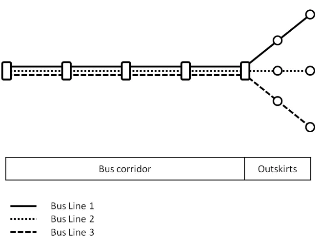
In order to develop a parametrical socio-economic cost-benefit analysis, we design a stylised model of a quite usual urban situation where an upgrade towards a light rail system could be considered.

Let’s consider an urban path where different bus lines superpose their

Figure 1 – Schematic representation of the stylised network

Anyhow, the level of service obtained with buses in this way could be unsatisfactory because of some factors. For example, it could be that bus lines, having too long paths, could become unreliable and generate delays8.

In such cases, an upgrade towards a Light Rail system on the corridor could be considered9 (see Errore. L'origine riferimento non è stata trovata.), in order to improve the quality of the service. Obviously, the division of formerly unique lines is introducing an interchange that breaks the direct connection between the outskirts and the corridor (and likely the town centre).

8

Among the most quoted motivations of preference for LR instead of BRT: low reliability, lower comfort, difficult boarding, congestion at bus stops for high frequency services, difficulty in prioritisation at junctions, etc.

9

Figure 2 - Schematic representation of the stylised network, after the introduction of a light rail on the corridor. Users coming from the outskirts, where bus service is kept, will need to make an interchange.

As first element of the model, we introduce the parameters in Table 1 in order to describe the demand.

Table 1 - Demand parameters

Parameter Description Unit

Q total current users that will use the light rail Mpax/year f part of total current users Q that will suffer

the modal interchange

0 ÷ 1, proportional to Q θ fixed relative rate of demand growth per

year

%

n new demand on the light rail, both generated and diverted from cars

0 ÷ 1, proportional to

Q·(1-f) * Modal

* We assume that the only part of the current demand Q that will increase after the introduction of the LR is the one that will not suffer a new interchange, which is

Q·(1-f)

To the f share of users is associated a cost of interchange. As will be shown, this interchange cost is one of the key factors for success or un-success of these systems.

5.

The parametrical socio-economic cost-benefit analysis

A parametrical socio-economic cost-benefit analysis of the stylised model introduced in the former section can help in deriving some reflections about the circumstances in which light rail schemes can be truly convenient from a socio-economic point of view. This section will describe the parameters or benefit&cost descriptors to be modelled.

Macroeconomic parameters

Among the macroeconomic and general inputs of CBAs, the ones more significant are the social discount rate and the length of the analysis (see Table 2).

Table 2 – Cost-benefit analysis parameters (source: DG REGIO, 2008)

Parameter Description Suggested values

r social discount rate 3,5% for EU non- Cohesion countries, 5.5% for EU Cohesion countries

T time horizon 30 years

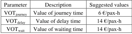
A common parameter is the value of time, that literature usually specifies in different situations (see Table 3).

Table 3 – Values of time for light rail users (our elaboration based on source: DG REGIO, 2008 and DfT, 2010)

Parameter Description Suggested values VOTjourney Value of journey time 6 €/pax-h

VOTdelay Value of delay time 14 €/pax-h

Investment cost

LRs (Knowles, 2007; SDG, 2005) usually require high investment costs, even if generally lower than heavy rail or underground metros. Common values range from 6 M€ to 30 M€10 for a two way route-km. Bus lanes are considerably cheaper, ranging from 350 k€ to 700 k€ for simpler solutions to 1.2 M€ to 2.5 M€ for prioritised circulation. Totally segregated busways investment costs seem to be much variable (1.2 M€ - 25 M€).

We introduce also the residual value (RV) at the end of the analysis period. Considering a 30 years horizon, we set it equal to the 50% of the investment (as suggested for railways for example by DG REGIO, 2008) and actualised at the last year of analysis:

Parameter Description Unit

I Total investment costs M€

RV _{Residual value of the investment at the Tth year:}

) (

5

,

0

)

1

(

5

,

0

T

I

e

r

I

RV

M€

We prefer not to introduce investment cost per km for two reasons. Firstly, because this makes much simpler the following calculations. Secondly because it makes easier and more significant the use of our formula. In fact, the cost per km is not always significant and representative of the variety of situations11, while the total cost is always known (or estimated) when introducing a new system.

Fixed maintenance and operating costs

Maintenance and operating costs are very important in order to assess the case for upgrading towards a light rail systems. In general, fixed maintenance costs of the systems tend to be higher for LRs, because of the

10

Some of the values suggested in those papers are taken from British sources; the exchange rate of British Pound (GBP) with respect to Euro (EUR) has changed a lot in recent years, ranging from 1 GBP for 1.45 EUR in 2007 to 1 GBP = 1.11 EUR in January 2010. In this paper we use a medium exchange rate of 1 GBP = 1.2 EUR.

11

presence of a specific infrastructure, while operating unit costs decrease with patronage much faster for LRs than for buses. Maintenance costs can be considered as fixed, and for railways the literature suggests them to be of the order of 1% of the investment costs, per year (de Rus and Nash, 2007; Baumgartner, 2001). In order to simplify, fixed maintenance costs are ignored for bus systems (see Table 4).

Table 4 – Fixed maintenance costs assessment parameters

Parameter Description Suggested values

Cfm, bus Bus line fixed maintenance costs ~ 0 M€/year

Cfm, LR LR line fixed maintenance costs:

I

C

0

.

01

,

in M€/year

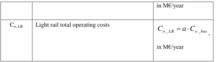
In this model we define the LR operating as a share of the bus ones,

which we assume to be of the order of 0.75 €/pax-km12 (see Table 5). For simplicity in calculations, we consider the total operating cost, depending both on per km costs and number of km produced. In fact, if the LR allows savings due to reduced frequency, those should be included here13.

Table 5 – Total operating costs assessment parameters

Parameter Description Suggested values

a Percentage of light rail operating costs with respect to bus ones

Co, bus Bus line total operating costs

Q

C

0

.

75

,

12_{If we consider a 20 km bus line with common European operating costs of 3 €/vehic}

-km and a frequency of 10 minutes per direction we obtain operating costs of 4 M€/year. With an average load factor of 35% this line should move some 3 million passenger per year, giving

a unit operating cost of 0.75 €/pax-km.

13

in M€/year

Co, LR Light rail total operating costs

bus o LR

o

a

C

C

,

in M€/year

Modal shift

Diverting users from cars to public transport is one of the major goals of the introduction of a new system, because allows a reduction in external costs.

We introduce the parameters in Table 6 to assess the benefits from modal shift.

Table 6 - Modal shift assessment parameters

Parameter Description Suggested values

Δcext External unit cost savings, without congestion 0.053 €/pax-km*

cext_cong Congestion external unit costs (urban dense

traffic)

2.1 €/pax km**

dcc Percentage of traffic under dense congestion conditions

that diverted users used to suffer***

0.20

l Average trip length [km] km

p Demand diverted from cars**** with respect to new demand n

0 ÷ 1

* Source: INFRAS-IWW, 2004

** Our elaboration (2.7 €/veickm with car load factor = 1.3) based on source: INFRAS-IWW,2004

*** The English WebTag tool (Dft,2010) reports 18.7% of congestion levels 4 and 5 in non-London UK cities

**** For example, NAO (2004) and Bottoms (2003) report a modal shift of 18% -20%

l

dcc

c

c

b

(

)

, [€/pax]

First year expected benefits from modal shift will be:

) 1 ( f Q n p b

B_{MS MS}

, [M€/year]

Improved regularity

As already said in the previous section, the introduction of light rail transit can improve the regularity of the systems, in terms of delay savings and affordability with respect to the timetable.

In instances where, for example (SDG, 2005), total bus service reaches levels of around 60 per hour, bus journey times are typically affected by delays as it is not possible to provide junction priority for all of the buses. Congestion may also occur at bus stops on route and in city centres.

We introduce the parameters in Table 7 to assess the benefits from improved regularity. Obviously this benefit can be existing or not according to cases.

Table 7 – Improved regularity assessment parameters

Parameter Description Suggested values VOTdelay Value of delay time 14 €/pax-h

d Average delay savings [min]

The expected unit benefit from improved regularity will be:

delay

reg

VOT

d

b

60

, [€/pax]

First year expected benefits from improved regularity are then evaluated, using the rule of half for the new demand (DG REGIO, 2008):

)

1

(

2

1

f

Q

n

b

Q

b

Reduction of the frequency of the service

LR can provide the same amount of seats with a reduced number of vehicles with respect to buses. This means that there could be a reduction in the frequency of the service, which represents a cost for the users.

We propose that a reduction in the frequency generates a cost which is half the increase of the headway (h)14. In fact, if a user wants to reach his destination at a defined hour, he will need to be there with an advance that can vary from 0 to h, depending on the timetable. So users will need to arrive at their destinations on average with an advance of h/2. If the headway of the service increases from hbus to hLR, the cost of this increase

will be half the increase itself.

We introduce the parameters in Table 8 to assess the cost from reduction of the frequency of the service.

Table 8 – Frequency of the service assessment parameters

Parameter Description Suggested values

Y Equivalent days per year 300 days/year

CAPbus Bus vehicle capacity 75 – 125

pax/vehicle CAPLR Light rail vehicle capacity 250 pax/vehicle

PhF Peak hour to day expansion factor (both directions)

9 times

LF Average peak hour load factor 0.8 (80%)

VOTwait Value of waiting time 14 €/pax-h

The headway of the service depends on the capacity of the chosen vehicles. Capacity of bus vehicles ranges from 75 people for standard buses to 125 people for articulated buses. Trams and LR capacity varies significantly; we chose for the exemplification a tram that can bring 250 users, The needed headway to carry a given demand is15:

14

Headway is the time distance between two trains or buses and is the inverse of the frequency.

15

6

10

2

Q

LF

CAP

PhF

Y

h

bus

, [hours]

6

10

2

Q

LF

CAP

PhF

Y

h

LR

, [hours]

The expected unit costs from the reduction of frequency will be:

wait bus

LR

freq

h

h

VOT

c

2

1

, [€/pax]

First year expected waiting time costs from the reduction of frequency are then evaluated , using the rule of half for the new demand (DG REGIO, 2008):

)

1

(

2

1

f

Q

n

c

Q

c

C

, [M€/year]

Interchange costs

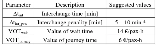
As already mentioned, the introduction of an interchange represents a cost for some users. The literature and guidelines (TRL, 2004; DfT, 2010) suggest to assess the cost of the interchange measuring the extra-time needed to get off the bus, get on the train and the unavoidable wait time, plus an interchange penalty to take into account the discomfort of the operation. This penalty is assessed as additional journey time.

We introduce the parameters in Table 9 to assess the costs from forced interchange.

Table 9 – Interchange assessment parameters

Parameter Description Suggested values Δtint Interchange time [min]

Δtint_pen Interchange penality [min] 5 – 10 min *

VOTwait Value of wait time 14 €/pax-h

* Source: TRL, 2004

The expected unit costs from forced interchange will be:

journey pen wait IC

VOT

t

VOT

t

c

60

60

int

, [€/pax]

First year expected costs from the reduction of frequency, applied to the users who suffer the new interchange (which is f·Q), are then evaluated:

Q f c

C_{IC IC}

, [M€/year]

Total actualised costs and benefits and NPV

The expected costs and benefits at each year have to be summed up, actualised at year 0 and, if the case, increased with the growth of the demand.

Demand grows with a fixed relative rate θ, so the value of Q at year t is:

t e Q t Q( )

The actualisation of costs and benefit at year 0 from year t, can be well approximated with an exponential form:

t r

t B e

r B t B ) 1 ( )

(

;

t C e

r C t C ) 1 ( ) (

The total actualised costs of the light rail scheme introduction will then be: T t r bus o LR o T rt bus fm LR fm

TOT

I

RV

C

C

e

dt

C

Q

C

Q

e

dt

C

(

)

(

)

, in

M€

The total actualised benefits of the light rail scheme introduction will be: T t r IC freq speed reb MS

TOT

B

Q

B

Q

B

Q

C

Q

C

Q

e

dt

B

)

(

)

(

)

(

)

(

)

(

,

in M€

At the end, the Net Present Value of the introduction of a light rail scheme on the present bus corridor is:

TOT

TOT C

B NPV

To know the maximum investment I that can be justified by the total present demand Q we solved the equation NPV = 0 with respect to I.

6.

Results

The above described model can be used to calculate synthetically a Net Present Value of the substitution of a previous situation characterised by continuous bus lines with a new network configuration of better characteristics (capacity, running costs, speed, etc.). This new configuration forces users coming by bus from the outskirts to interchange to another high frequency system running on the common part of former bus lines. The common part can be exercised with high capacity vehicles (being it a tramway, a light rail or even a bus line) and can be segregated and/or prioritised in order to obtain a higher commercial speed. Also in this case the same result, if geometrically possible in the analysed city, could be theoretically provided with buses.

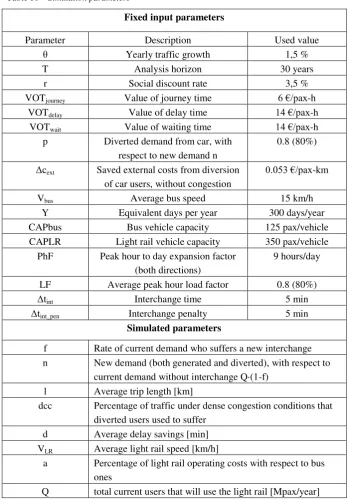
Table 10 – Simulation parameters

Fixed input parameters

Parameter Description Used value

θ Yearly traffic growth 1,5 %

T Analysis horizon 30 years

r Social discount rate 3,5 %

VOTjourney Value of journey time 6 €/pax-h

VOTdelay Value of delay time 14 €/pax-h

VOTwait Value of waiting time 14 €/pax-h

p Diverted demand from car, with respect to new demand n

0.8 (80%)

Δcext Saved external costs from diversion

of car users, without congestion

0.053 €/pax-km

Vbus Average bus speed 15 km/h

Y Equivalent days per year 300 days/year

CAPbus Bus vehicle capacity 125 pax/vehicle

CAPLR Light rail vehicle capacity 350 pax/vehicle PhF Peak hour to day expansion factor

(both directions)

9 hours/day

LF Average peak hour load factor 0.8 (80%)

Δtint Interchange time 5 min

Δtint_pen Interchange penalty 5 min

Simulated parameters

f Rate of current demand who suffers a new interchange n New demand (both generated and diverted), with respect to

current demand without interchange Q·(1-f) l Average trip length [km]

dcc Percentage of traffic under dense congestion conditions that diverted users used to suffer

d Average delay savings [min] VLR Average light rail speed [km/h]

a Percentage of light rail operating costs with respect to bus ones

In the next pages we draw diagrams representing three variables among the eight listed above and fixing the other five.

We limited the variability to these variables only for simplicity’s sake

and because we think that these are the significant ones when taking a decision. For example, a tram system could be similar for users if the interchange cost equals the higher commercial speed; in this case the substitution of the existing bus system with a costly tram can be justified if running costs are lower. Our diagram will tell us for which demand level in Mpax/year, the designed system (and the consequent needed investment) can be socially desirable.

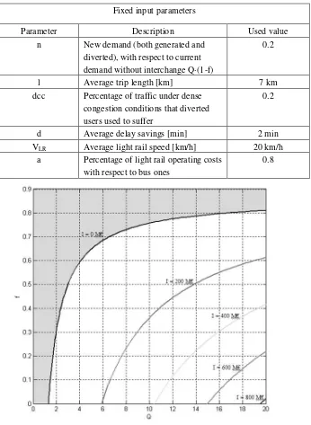
Because of the importance of the parameter f (rate of current demand who suffers a new interchange), we represent the respective abacus for three different level of light rail running costs with respect to bus ones (a = 0.4, a = 0.8 and a = 1.2). All other abaci will be calculated only for

Figure 1 – I(Q,f): Justified investment (I) with respect to current demand on the corridor (Q, in Mpax/year) and rate of users affected by a new interchange (f). Grey area represents circumstances in which no investment is justified.

Fixed input parameters

Parameter Description Used value

n New demand (both generated and diverted), with respect to current demand without interchange Q·(1-f)

0.2

l Average trip length [km] 7 km

dcc Percentage of traffic under dense congestion conditions that diverted users used to suffer

0.2

d Average delay savings [min] 2 min

VLR Average light rail speed [km/h] 20 km/h

a Percentage of light rail operating costs with respect to bus ones

Figure 2 – I(Q,f,a): Justified investment (I) with respect to current demand on the corridor (Q, in Mpax/year) and rate of users affected by a new interchange (f). On the left the abacus is calculated with a=0.4, on the right using a=1.2. Grey area represents circumstances in which no investment is justified.

Fixed input parameters

Parameter Description Used value

n New demand (both generated and diverted), with respect to current demand without interchange Q·(1-f)

0.2

l Average trip length [km] 7 km

dcc Percentage of traffic under dense congestion conditions that diverted users used to suffer

0.2

d Average delay savings [min] 2 min

VLR Average light rail speed [km/h] 20 km/h

a Percentage of light rail operating costs with respect to bus ones

Figure 3 – I(Q,a): Justified investment (I) with respect to current demand on the corridor (Q, in Mpax/year) and light rail operating costs with respect to bus ones (a)

Fixed input parameters

Parameter Description Used value

f Rate of current demand who suffers a new interchange

0.3

n New demand (both generated and diverted), with respect to current demand without interchange Q·(1-f)

0.2

l Average trip length [km] 7 km

dcc Percentage of traffic under dense congestion conditions that diverted users used to suffer

0.2

d Average delay savings [min] 2 min

Figure 4 – I(Q,n): justified investment (I) with respect to current demand on the corridor (Q, in Mpax/year) and new demand (both generated and diverted, n)

Fixed input parameters

Parameter Description Used value

f Rate of current demand who suffers a new interchange

0.3

l Average trip length [km] 7 km

dcc Percentage of traffic under dense congestion conditions that diverted users used to suffer

0.2

d Average delay savings [min] 2 min

VLR Average light rail speed [km/h] 20 km/h

a Percentage of light rail operating costs with respect to bus ones

Figure 5 – I(Q,l): Justified investment (I) with respect to current demand on the corridor (Q, in Mpax/year) and average trip lenght (l)

Fixed input parameters

Parameter Description Used value

f Rate of current demand who suffers a new interchange

0.3

n New demand (both generated and diverted), with respect to current demand without interchange Q·(1-f)

0.2

dcc Percentage of traffic under dense congestion conditions that diverted users used to suffer

0.2

d Average delay savings [min] 2 min

VLR Average light rail speed [km/h] 20 km/h

a Percentage of light rail operating costs with respect to bus ones

Figure 6 – I(Q,dcc): Justified investment (I) with respect to current demand on the corridor (Q, in Mpax/year) and percentage of traffic under dense congestion conditions that diverted users used to suffer (dcc)

Fixed input parameters

Parameter Description Used value

f Rate of current demand who suffers a new interchange

0.3

n New demand (both generated and diverted), with respect to current demand without interchange Q·(1-f)

0.2

l Average trip length [km] 7 km

d Average delay savings [min] 2 min

VLR Average light rail speed [km/h] 20 km/h

a Percentage of light rail operating costs with respect to bus ones

Figure 7 – I(Q,d) Justified investment (I) with respect to current demand on the corridor (Q, in Mpax/year) and average delay savings suffer (d, in minutes)

Fixed input parameters

Parameter Description Used value

f Rate of current demand who suffers a new interchange

0.3

n New demand (both generated and diverted), with respect to current demand without interchange Q·(1-f)

0.2

l Average trip length [km] 7 km

dcc Percentage of traffic under dense congestion conditions that diverted users used to suffer

0.2

VLR Average light rail speed [km/h] 20 km/h

a Percentage of light rail operating costs with respect to bus ones

Figure 8 – I(Q,VLR): Justified investment (I) with respect to current demand on the corridor

(Q, in Mpax/year) and average light rail speed (VLR, in km/h)

Fixed input parameters

Parameter Description Used value

f Rate of current demand who suffers a new interchange

0.3

n New demand (both generated and diverted), with respect to current demand without interchange Q·(1-f)

0.2

l Average trip length [km] 7 km

dcc Percentage of traffic under dense congestion conditions that diverted users used to suffer

0.2

d Average delay savings [min] 2 min

a Percentage of light rail operating costs with respect to bus ones

7.

Conclusions

The choice of upgrading a simple bus system with a hierarchical system based on external bus lines feeding one central high capacity corridor has been often at stake for local administrations. In Europe, when this decision is taken, the system chosen for the high capacity segment is usually LR (being it tram or metro). In the rest of the world the completely different city structure suggested in many cases to focus on less expensive but more space consuming BRT.

Whatever is the choice from a urban design viewpoint, the main problem is to rationally evaluate all the complex variables influencing the choice: the expected demand, the modal shift, the length of the line, the commercial speed, etc. In this paper we realised a simplified cost-benefit model in order to point out the influence of the main design variables on the social desirability of the upgrade. Many of these variables are very important, but quite easy to find in literature, for example the value of time. To try to give a general answer, we chose one single value for these variables, conscious that a real world analysis must pay a lot of attention also to these parameters. To simplify calculations and to make the use of the abaci easier, we decided to refer to total investment and operating costs and not to unitary costs. For example, we do not draw abaci in function of investment cost per km or operating cost per vehicle*km because these parameters are deeply influenced by local conditions and by design choices. The meaning of our simulations is then to find the switch values that makes a project feasible. For example, at a given total demand and other characteristics, the scheme is feasible if its total cost is above a certain level of variables, independently from the length of the line.

After fixing these parameters, we isolated the design characteristics that we consider as the most relevant:

The existing demand (Q)

The share of Q demand subject to interchange (f)

The percentage of generated demand (n) with respect to Q

The average trip length (l)

The average delay savings thanks to higher reliability of guided systems (d)

The LR commercial speed compared to a bus commercial speed of 15 km/h (VLR)

The total investment cost (I)

We ran simulations of these parameters and drew some abaci to help the decision maker in the calculus of the magnitude orders of the switch values. Of course, many other relationships among variables could be explored trough other abaci, but results and conclusions are still quite clear:

a)The new (generated and diverted) demand (n) is important only in case of extreme congestions (high dcc). When the demand diverted from cars is around 20% (a typical situation), dcc

influences slightly the results.

b)The demand subject to interchange (f) is always important due to the penalty caused by interchange costs (typically 5+5 min). When the share is high, namely when the LR is substituting the previous bus lines only in the central part of the city and users are subject to interchange when coming from outskirts, the

“captive” demand of the central part of the line (Q) must be very high (for example, above 14 Mpax/year if I=200M€).

c)When demand is high, moving from a low capacity system (bus) to one characterised by higher capacity (LR) can lower the total operating costs (independently from the unit operating cost that can be higher or lower according to the chosen system, there should be a reduction of bus*km ran). The variable describing the ratio between costs (a) is extremely significant.

d)When average trip length (l) is short, LR is justified only if extremely cheap.

e)Below 6 Mpax/year LR systems are feasible only under very peculiar conditions: cost less than 200 M€ and no interchange users, or generated demand above 50% of the total, or trip length above 10km, or more than 50% of streets under dense or severe congestion conditions, or commercial speed above 25km/h, or extreme reduction in operating costs.

15km, or severe road congestion for 80% of streets and hours of the day, or extremely fast systems above 30 km/h.

In conclusion, we demonstrated that there are many interesting conditions under which LR or BRT are applicable, but only if the cost is kept low, i.e. for lighter solutions. However, comparing the results with many real world cases we see numerous cities where LR was not necessary at all, being this technical solution chosen for small traffic volumes and since often its construction is not associated to cost savings due to network rationalisation. In cities (or corridors) with no dense congestion for many hours of the day, similar levels of service can be supplied with normal buses, sometimes even better because no interchange is needed. Similarly, corridors with low demand (of few millions passengers) do not need any track improvement. Excellent results could be obtained simply caring of vehicles quality, waiting time, comfort at stops, good interchanges between lines.

References

Balcombe et al. (2004), The demand for public transport: a practical guide, TRL Report, Crowthorne (UK)

Baumgartner J. P. (2001), Prices and costs in the railways sector, Laboratoire d’Intermodalité des Trasports et de Planification, École Polytechnique Fédérale de Lausanne, Losanne (CH)

Bottoms G. D. (2003), =Continuing Developments in Light Rail Transit in Western Europe. United Kingdom, France, Spain, Portugal, and Italy”, Transportation Research E-Circular, p. 713-728, Transportation Research Board, Washington, DC (USA).

de Rus G., Nash, C. A. (2007), In what circumstances is investment in HSR worthwhile?, Institute for Transport Studies, University of Leeds (UK).

de Rus J., Nombela G. (2007), “Is Investment in High Speed Rail Socially Profitable?”, Journal of Transport Economics and Policy, Vol. 41, Part 1, 3 - 23.

DfT (2010), Transport Analysis Guidance – WebTAG, Department for Transport, London (UK).

DG REGIO (2008), Guide to Cost Benefit Analysis of investment Projects, Directorate General Regional Policy, European Commission.

Henry, L., Litman, T. A. (2006), Evaluating New Start Transit Program Performance, Comparing Rail And Bus, Victoria Transport Policy Institute, website: www.vtpi.org, Victoria, BC, Canada.

Hensher, D. A. (1999), “A bus-based transitway or light rail? Continuing the saga on choice versus blind commitment”, Road & Transport Research, Vol 8, No 3, September 1999.

Knowles, R. D.(2007), “What future for light rail in the UK after Ten Year Transport Plan targets are scrapper?”, Transport Policy, 14 (2007), pp. 81-93, Elsevier

Litman, T. A. (2010), Evaluating Public Transport Benefits and Costs, Best Practices Guidebook, Victoria Transport Policy Institute, website: www.vtpi.org, Victoria, BC, Canada.

NAO (2004), Improving public transport in England through light rail, National Audit Office, Report by the comptroller and auditor general, HC 518 Session 2003-2004:23 April 2004, Ordered by the House of Commons, London (UK) Nair, P. and Kumar, D. (2005), “Transformation in Road Transport System in

Bogota: An Overview”, The ICFAI Journal of Infrastructure, September 2005 Pinheiro, C. (2005), “Curitiba, una experiencia continua en soluciones de

transporte”, The European Journal of Planning

Rathwell, S. and Schijns, S. (2002), “Ottawa and Brisbane: comparing a mature busway system”, Journal of Public Transportation, Volume 5, n. 2, pp. 163 - 182.

TfL (2004), West London Tram Project (WLT), Board Paper presented at the Board Meeting Agenda hold on 29th April 2004 in the Chamber, City Hall of London (UK).

SDG (2005), What light rail can do for cities, A Review of the Evidence, Final Report, Steer Davies Gleave, Prepared for PTEG – Passenger Transport Executive Group, London (UK)