Munich Personal RePEc Archive
The impact of real oil price on real
effective exchange rate: The case of
Azerbaijan
Hasanov, Fakhri
Institute for Scientific Research on Economic Reforms, DIW Berlin
(German Institute for Economic Research)
July 2010
Online at
https://mpra.ub.uni-muenchen.de/33493/
Deutsches Institut für Wirtschaftsforschung
www.diw.de
Fakhri Hasanov
Berlin, August 2010
The Impact of Real Oil Price on Real
Effective Exchange Rate:
The Case of Azerbaijan
1041
Opinions expressed in this paper are those of the author(s) and do not necessarily reflect views of the institute.
IMPRESSUM
© DIW Berlin, 2010
DIW Berlin
German Institute for Economic Research Mohrenstr. 58
10117 Berlin
Tel. +49 (30) 897 89-0 Fax +49 (30) 897 89-200
http://www.diw.de
ISSN print edition 1433-0210 ISSN electronic edition 1619-4535
Papers can be downloaded free of charge from the DIW Berlin website:
http://www.diw.de/discussionpapers
Discussion Papers of DIW Berlin are indexed in RePEc and SSRN:
http://ideas.repec.org/s/diw/diwwpp.html
1
The Impact of Real Oil Price on Real Effective Exchange Rate:
The Case of Azerbaijan
Fakhri Hasanov
1Abstract:
Using quarterly data from 2000-2007 and applying Error Correction Model and Johansen
Co-integration Approaches I estimate the impact of real oil price on the real exchange rate of
Azerbaijani manat. Estimation outputs derived from these approaches are very close to each other
and indicate that real oil price has statistically significant positive impact on real exchange rate in
the long-run. Besides, revealed that relative price as a proxy for productivity has also explanatory
power in explaining long-run behavior of real exchange rate. Estimated Error Correction Term
indicates that half-life of adjustment toward long-run equilibrium level takes 3-4 quarters. Since
findings of this study occur as results of high fiscal expansion my policy suggestions mainly related
to Fiscal policy implementations.
Keywords:
Real effective exchange rate, Real oil price, Relative productivity, Azerbaijani manat, Dutch
Disease, Oil-exporting Countries, Johansen Co-integration Approach, Error Correction Modeling,
Half-life Speed.
JEL:
F31, F41, C32, P24, Q43
1
CONTENT
Introduction ... 3
Literature review ... 5
Methodology and Data ... 7
Real Exchange Rate Equation... 7
Econometric Methodology... 9
Data... 12
Estimation Outputs ... 14
Interpretations of Estimation Results... 17
Conclusion and Policy Suggestions ... 18
References ... 19
3
Introduction
Azerbaijani economy has performed rapid economic development approximately since 2004. It is obvious
that this economic development mainly sourced from oil sector of economy. Oil extraction and exportation,
also increasing oil prices in the world markets cause huge inflow of oil revenues into countries. These oil
revenues have certain effect on macroeconomic performance of Azerbaijan. For example, GDP growth rate
was 34.5% in 2006 which made country a leader in the world in terms of growth rates; money supply has
increased more than two times in 2006 and 2007 and one can observe high inflation rates starting from 2004.
In parallel with above mentioned performance at the same time Azerbaijani economy faces sustainable
appreciation of exchange rate, which undermines competitiveness of non-oil sector of economy. I assume
that this permanent appreciation is tightly related to oil price and subsequently oil revenues. There are at
least three reasons that allow us to think so.
First of all, resource curse concept, especially Dutch Disease phenomenon predicts certain link between
appreciation of real exchange rate and resource price [Corden and Neary (1982), Corden (1984), Wijnbergen
(1984), Buiter and Purvis (1982), Bruno and Sachs (1982), Enders and Herberg (1983), Edwards (1985)].
According to theoretical framework of Dutch Disease, there are three theoretical reasons why the relative
price of non-tradable and therefore overall price level may rise [Egert (2009), Algozina (2006)]. The first
reason is related to non-tradable prices raise due to leaves labour out of non-tradable sector. The second is
that higher productivity in commodity sector that pushes up wages in the commodity sector which leads to
higher wages in the non-tradable sector and, consequently, to higher non-tradable prices or consumer price
level. Third, the relative price of tradable raises to the event that higher profits and wages in the
non-tradable and the related tax revenues are spent on non-non-tradable goods and provided the income elasticity of
demand for non-tradable is positive.
Secondly, there are number of empirical studies that investigate impact of oil price on real exchange rate and
find positive relationship between them in the oil exporting countries Koranchelian (2005) in Algeria;
Zalduendo (2006) in Venezuela; Issa et al. (2006) in Canada; Habib and Kalamova (2007) in Norway, Saudi
Arabia and Russia, Oomes and Kalcheva (2007) in Russia; Korhonen and Juurikkala (2009) in nine OPEC
countries; Jahan-Parvar and Mohammadi (2008) in fourteen oil-exporting countries.
to non-tradable sector of economy as budget expenditures. These expenditures generate spending effect and
result increase of relative price in non-tradable sector therefore, high inflation rates. On another side before
spending, these revenues have to be converted into national currency which leads to excess supply of foreign
currency and therefore, appreciation of nominal exchange rate. As a result, appreciation of real exchange rate
sources from both channels, i.e. through rise in relative prices and appreciation in nominal exchange rate.
Since Azerbaijan is oil-exporting country and its economy experiences appreciation of real exchange rate it
is important to analyze that whether this appreciation is mainly sourced from oil prices or not. Therefore,
objective of this study is to investigate impact of real oil price on real exchange rate.
By conducting this study I can answer the following research question: Does real oil price play any role in
formation of equilibrium path of real exchange rate?
Thus, based on theoretical framework of Dutch Disease [Corden and Neary (1982), Corden (1984)] and by
following above mentioned empirical studies especially Jahan-Parvar and Mohammadi (2008), Koranchelian
(2005), Zalduendo (2006), Habib and Kalamova (2007), Oomes and Kalcheva (2007), Korhonen and Juurikkala
(2009) I analyze impact of real oil price on real exchange rate of Azerbaijani manat. I have found that there is
statistically significant and positive relationship between the real oil price and real exchange rate over the research
period. It is important to note that we cannot conclude that Azerbaijani economy has contracted Dutch Disease
just by estimating impact of real oil prices on real exchange rates and in this regard we have to check all
symptoms of Dutch Disease in parallel with carefully testing alternative explanations of observed processes.
Results of the study may be useful for policymakers in terms of policy implementation related to
management of oil revenues and exchange rate policy. On another side this paper is the pioneer study in the
area of investigation of relationship between oil price and real exchange rate in Azerbaijan.
The rest part of the paper is organized as below. Review of appropriate theoretical and empirical literatures
are given in Literature Review section, while Methodology and Data section consists of employed
econometric methodology and required data. Estimation Outputs section comprises results of econometric
estimations and their interpretations are reflected in Interpretation of Estimation Results section. Main
findings of the study and proposing policy recommendation are discussed in Conclusion and Policy
Suggestion section. Reference section consists of list of reviewed literatures. Estimation outputs and graphic
illustrations are presented in Appendix.
5
Literature review
Since my research direction is narrow, i.e. the investigation of impact of real oil price on real exchange rate I
should mainly focus on such kinds of literatures rather than studies relating assessment of equilibrium real
exchange rate in general. Therefore, I review some theoretical and empirical studies that investigate the
impact of real oil price on real exchange rate in oil exporting countries. Theoretical base of such kinds of
investigations come from Dutch Disease Theory, one of the resource curse concepts. According to Corden
(1982) and Corden and Nearly (1984) Dutch Disease is the appreciation of a country’s real exchange rate
caused by an exogenous increase in resource price or sharp rise in resource export and the tendency of a
booming resource sector to draw capital and labour away from a country’s manufacturing and agricultural
sectors, which can lead to a decline in exports of these sectors and inflate the cost of non-tradable goods2.
Some theoretical aspects of Dutch Disease have been developed by also Wijnbergen (1984), Buiter and
Purvis (1982), Bruno and Sachs (1982), Enders and Herberg (1983), Edwards (1985) and etc. According to
theoretical framework of Dutch Disease, there are three theoretical reasons why the relative price of
non-tradable, therefore, overall price level and subsequently real exchange rate may rise [Egert (2009), Algozina
(2006)]. The first reason is related to non-tradable prices raise due to leaves labour out of non-tradable
sector. The second higher productivity in commodity sector pushes up wages in the commodity sector which
leads to higher wages in the non-tradable sector and, consequently, to higher non-tradable prices or consumer
price level. Third, the relative price of non-tradable raises to the event that higher profits and wages in the
non-tradable and the related tax revenues are spent on non-tradable goods and provided the income elasticity
of demand for non-tradable is positive.
Regarding with empirical literatures, there are number of studies that investigate the impact of real oil price
2
on real exchange rate in oil exporting country or country groups.
Koranchelian (2005) investigates the impact of real oil price and Real GDP per capita relative to trading
partners as a proxy for relative productivity on Algerian real effective exchange rate by employed VECM
approach over the annual period of 1970-2003. Author reveals that real oil price together with relative
productivity has statistically significant and positive impact on real effective exchange rate.
Zalduendo (2006) examines co-integration relationship between CPI-based real effective exchange rate and real
oil price, relative productivity, government expenditure as a share of GDP and differential in real interest rates
over the period of 1950-2007 by using VECM. His main findings are that (a) oil prices have indeed played a
significant role in determining a time-varying equilibrium real exchange rate path; (b) oil prices are not the
only important determinant of the real effective exchange rate: declining productivity is also a key factor; (c)
appreciation pressures are rising; (d) the speed of convergence is higher.
Issa et al. (2006) revisits the relationship between energy prices and the Canadian dollar over the 1973–2005
in the Amano and van Norden (1995) equation, which shows a negative relationship such that higher real
energy prices lead to a depreciation of the Canadian dollar. Based on structural break tests, the authors find a
break point in the sign of this relationship, which changes from negative to positive in the early 1990s. The
break in the effect between energy prices and the Canadian dollar is consistent with major changes in
energy-related cross-border trade and in Canada’s energy policies.
Habib and Kalamova (2007) investigate whether the real oil price and productivity differentials against 15
OECD countries have an impact on the real exchange rates of three main oil-exporting countries: Norway and
Saudi Arabia (in the period of 1980-2006) and for Russia (in the period of 1995-2006). In the case of Russia it
is possible to establish a positive long-run relationship between the real oil price and the real exchange rate.
However, authors find virtually no impact of the real oil price on the real exchange rates of Norway and Saudi
Arabia. The diverse exchange rate regimes cannot help in explaining the different empirical results on the
impact of oil prices across countries, which instead might be due to other policy responses, namely the
accumulation of net foreign assets and their sterilization, and specific institutional characteristics.
Kalcheva and Oomes (2007) test symptoms of Dutch Disease, i.e. (1) real exchange rate appreciation; (2)
slower manufacturing growth; (3) faster service sector growth; and (4) higher overall wages while carefully
Main conclusion of this study is that Russia has all of the symptoms of which real oil price has statistically
significant and positive impact on real effective exchange rate in the long run.
Korhonen and Juurikkala (2009) assess the determinants of equilibrium real exchange rates in OPEC countries
over the period of 1975 to 2005. By utilizing pooled mean group and mean group estimators, authors find that the
price of oil has a clear, statistically significant effect on real exchange rates in oil producing countries in the
long-run. Higher oil price lead to appreciation of the real exchange rate. Elasticity of the real exchange rate with respect
to the oil price is typically between 0.4 and 0.5, but may be even larger depending on the specification. Real per
capita GDP, on the other hand, does not appear to have a clear effect on real exchange rate.
Jahan-Parvar and Mohammadi (2008) test the validity of the Dutch Disease hypothesis by examining the
relationship between real oil prices and real exchange rates in a sample of fourteen oil exporting countries
over the annual period of 1970-2007. Autoregressive distributed lag (ARDL) bounds tests of co-integration
support the existence of a stable relationship between real exchange rates and real oil prices in all countries,
suggesting a strong support for the Dutch Disease hypothesis.
By summarizing, all of these articles can be concluded that not depending on objective of the investigations,
i.e. testing Dutch Disease Hypothesis, or just measurement the impact of real oil price on real exchange rate
these studies reveal statistically significant positive impact of real oil prices on real exchange rate in
oil-exporting countries.
Methodology and Data
Real Exchange Rate Equation
For the estimation of real exchange rate I am going to use behavioral equilibrium exchange rate (BEER) approach
(Clark and MacDonald, 1998, 2000). This framework suggests looking for a long-run (co-integrating) relationship
between the real exchange rate and its economical fundamentals. The theoretical underpinning of the BEER
approach rests on the basic concept of uncovered interest rate parity (UIP):
*)
(
)
(
t 1 t tt
t
E
q
R
R
q
=
+−
−
(1)7
at time t,
R
t andR
t*
−
are domestic and foreign real interest rates at time t respectively.Under the BEER approach the unobservable expectation of real exchange (Et(qt+1)) is assumed to be
determined solely by a vector of long-run economic fundamentals Zt (Siregar and Rajan, 2006). It is
assumed that Zt vector mainly consists of three long run fundamentals namely the relative price of
non-traded to non-traded goods
(
NTT
)
as a proxy for relative productivity, net foreign assets(
NFA)
and terms oftrade
(
TOT
)
[Faruqee, (1995), MacDonald (1997), Stein (1999), Clark and MacDonald, (1998), Clark andMacDonald, (2000)]. Thus, the BEER approach produces the estimates of equilibrium real exchange rate
(
q
tREER) as a function of the long-run economic fundamentals and the short-run interest rate differentials:(
t t t t t)
REER
t
f
R
R
NTT
NFA
TOT
q
=
−
*,
,
,
(2)As state Korhonen and Juurikkala (2009) one of the privileges of BEER approach is that this approach can
take into account country specific features. So, I should make some changes in Equation (2) on the based on
Azerbaijani economy’s stylized facts:
a) Since financial market is weakly developed the interest rate differential can be dropped;
b) The studies such as Koranchelian (2005), Zalduendo (2006), Issa et al. (2006), Kalcheva and Oomes (2007),
Korhonen and Juurikkala (2007), Jahan-Parvar and Mohammadi (2008) examine relationship between oil price
and real exchange rate and reveal that oil prices have a significant impact on the real exchange rates in the
oil-exporting countries. Another side some determinants of real exchange rate such as terms of trade, net foreign
asset, government spending mainly depend on oil price in the oil-exporting economies. When the oil price raises
then terms of trade improves, net foreign assets increases, government expenditure expands and contrary as state
Habib and Kalamova (2007). Indeed in the case of Azerbaijan can be observed that there is higher correlation
between these above mentioned variables and oil price than real exchange rate. Hence I should exclude terms of
trade, net foreign asset from the Equation (2) by including real oil price (
OILP
r) here;So, after taking into account above mentioned stylized facts of Azerbaijani economy Equation (2) becomes
as following:
)
,
(
t trBEER
t
f
NTT
OILP
Note that such kind of specification as Equation (3) meets my research objective and is in line with research
specifications of Koranchelian (2005), Habib and Kalamova (2007), Korhonen and Juurikkala (2009). On
another side as indicates Rautava (2002) given the small number of observations, there is a need to keep the
system as small as possible in order to allow for the estimation of parameters.
Since the equilibrium rate is not an officially observable variable, a common empirical approach to estimate
the BEER involves two steps. The first step involves estimating the long-run (co-integration) relationship
between the prevailing real effective exchange rate (REER) and the economic fundamentals listed in
Equation (4):
r t t
REER
t
ntt
oilp
q
=
α
+
β
0+
β
1 (4)The second step uses the coefficient of these fundamental variables
(
α
ˆ
,
β
ˆ
0,
β
ˆ
1)
to compute the behavioralequilibrium exchange rate:
r t t
BEER
t
NTT
OILP
q
ˆ
=
α
ˆ
+
β
ˆ
0+
β
ˆ
1 (5)Econometric Methodology
Since I have small number of observation (only 31 observations) I intend to employ Autoregressive
Distributed Lag (ARDL) approach as main estimation methodology. At the same time in order to check
robustness of the results and juxtapose them I am going also to employ Johansen Co-integration Approach in
this study. ARDL approach has some advantages compared to other co-integration approaches [Pesaran et al.
(2001); Oteng və Frimpong (2006); Sulayman və Muhammad (2010)]: (a) ARDL approach is simple and can
be realized by using OLS; (b) There is no endogeneity problem in this method; (c) It is possible to estimate
long- and short-run coefficients in one equation simultaneously; (d) It is not needed to Test for Unit Root of
variables. In other words ARDL approach is irrespective whether variables in estimation are I(0) or I(1) or
mixture of them; (e) this approach is more effective than others when we have small number of observations.
ARDL approach consists of following procedures:
The first stage covers construction of unrestricted Error Correction Model (ECM)
t i t n
k i i
t n
k i t
yxx t
t
c
y
x
y
x
u
y
=
+
+
+
Δ
+
Δ
+
Δ
−= − =
−
−
0 1
1 1
1
0
θ
θ
ϖ
ϕ
(6)Where,
y
– is a depended variable;x
– stands for explanatory variables; - is a residuals of model, i.e.white noise errors; c0 – is a drift coefficients;
u
i
θ
- indicate long-run coefficients, whileϖ
iand
ϕ
i- reflectshort-run coefficients;
Δ
- is a difference operator;k
– is lag order.Note that coefficient on
y
t−1, i.e.
θ
1reflects error correction term.
Ifθ
1 is statistically significant andfalls interval of (-1:0) then can be considered that co-integration relationship between variables is stable. In
other words short run fluctation of variables corrects toward long-run equilibrium level.
It is worth to note that one of the main points in ARDL estmation is to correctly define lag order of the first
differenced variables. Because, finding co-integration relationship between variables is sensitive to lag order.
Optimal lag order in ARDL is usually defined by minimising of Akaike and Schwarz criteria and at the same
time removing serial autocorrelation of the residuals. Note that it is advisable to prefer Schwarz information
criterion in the case of small number of observations (Pesaran and Shin, 1997, p.4; Fatai and et. al, 2003, p.89).
After constructing proper ECM, the second stage is to test for existence of co-integration between variables. In
order to test for co-integration is used Wald-Test (or F-Test) on the
θ
i coefficients of Equation (6). Hullhypothesis is that there is no co-integration between variables (
θ
1=θ
2=θ
i= 0), while alternative hypothesis isthat there is co-integration between variables (
θ
1≠θ
2≠θ
i≠ 0)Note that F-statistics have non-standard distribution in the case of ARDL. Critical values of F distribution are
taken from specific table prepared by Pesaran and Pesaran and are reflected in Pesaran and Pesaran (1997) and
also Pesaran et. al (2001). The two sets of critical values provide critical value bounds for all classifications of
the regressors into purely I(1), purely I(0) or mutually cointegrated.
If the computed F statistics is higher than the upper bound of the critical values given significance level then the
null hypothesis of no cointegration is rejected. If the computed F statistics is smaller than the lower bound of
the critical values given significance level then the null hypothesis of no cointegration is accepted. The
co-integration test result is inconclusive if computed F statistics falls between upper and lower bands.
step of ARDL approach. Long-run coefficients can be calculated based on estimated Equation (6) by setting
1 1
0
+
y
t−+
yxxx
t−c
θ
θ
to zero and solving it fory
as following way:u
x
c
y
=
−
−
yxx+
θ
θ
θ
0
(7)
As I mentioned above in order to check robustness of the results and juxtapose them I am going also to employ
Johansen Co-integration Approach in this study. Johansen (1988) and Johansen and Juselius (1990) full
information maximum likelihood of a Vector Error Correction Model, which is as following:
t i t k i i t
t
y
y
y
=
Π
+
Γ
Δ
+
µ
+
ε
Δ
− − = −
1 1 1 (8)Where,
y
t is a (n x 1) vector of the n variables in interest,µ
is a (n x 1) vector of constants,Γ
represents a(n x (k-1)) matrix of short-run coefficients,
ε
tdenotes a (n x 1) vector of white noise residuals, andΠ
is a (nx n) coefficient matrix. If the matrix has reduced rank (0 < r < n), it can be split into a (n x r) matrix of
loading coefficients
Π
α
, and a (n x r) matrix of co-integrating vectorsβ
. The former indicates the importanceof the co-integration relationships in the individual equations of the system and of the speed of adjustment to
disequilibrium, while the latter represents the long-term equilibrium relationship, so that
Π
=
α
β
′
. K isnumber of lags; t denotes time and
Δ
is a difference operator.Testing for co-integration, using the Johansen’s reduced rank regression approach, centers on estimating the
matrix in an unrestricted form, and then testing whether the restriction implied by the reduced rank of
can be rejected. In particular, the number of the independent co-integrating vectors depends on the rank of
which in turn is determined by the number of its characteristic roots that different from zero. The test for
nonzero characteristic roots is conducted using Max and Trace
Π
Π
Π
3
tests statistics.
While the ARDL bound testing approach does not require pre-testing order of integration, all variables need to
be integrated of order one in order to apply the Johansen Co-integration method. Therefore, before estimating
the co-integrated vector-error correction by Johansen’s method, the stochastic properties of the data are
3 Since Trace tests tend to reject the null hypothesis of no co-integration in small samples, Johansen (2002) shows that as long as the
number of parameters per observation, kn/T (with k equal to the number of lags in VAR, n is the number of endogenous variables and
T is the length of the sample), is less than 0.20, the Trace test will give robust results. It is useful to take this ratio into account for our co-integration relationships because of we also have small numbers of observations.
assessed by menas of Unit-Root Tests. I am going to employ Augmented Dickey-Fuller (1981) and
Phillips-Perron (1988) unit root tests to assess the time-series properties of the data. The Augmented Dickey-Fuller
and Phillips-Perron tests maintain the null hypothesis of non-stationarity of the time series.
Data
Research covers quarterly data over the period 2000-2007 and includes: real effective exchange rate
(
REER
), domestic consumer price index (CPI), and domestic producer price index (PPI
), trade-weightedaverage consumer price index of main trading partners ( ), trade-weighted average producer price indices
of main trading partners (
F
CPI
F
PPI
) and manat-US Dollar bilateral exchange rate and nominal oil price.Real Effective Exchange Rate is a multilateral consumer price index based on real effective exchange
rate of a currency of domestic economy relative to its main trading partners. It is defined in terms of
foreign currency per unit of domestic currency, so that an increase in real effective exchange rate means
appreciation of domestic currency. Real effective rates are calculated by Central Bank of Azerbaijan
(CBA) and it can be retrieved from CBA official web-site (www.nba.az).
The Relative Price of Non-Traded to Traded Goods. This variable is used as a proxy for productivity
differentials4.
Productivity differentials are used to capture the Balassa-Samuelson effect5 that is one of main determinants
of real exchange rate. Ideally, direct measurements of productivity in the tradable and non-tradable sectors
should be used. However, such kind of data I could not find for Azerbaijan and its main trading partners. So,
two kinds of proxies can be used for measuring productivity differentials: The first one is the relative price of
non-tradable to tradable; a measurement employed by Macdonald (1997a) Clark and MacDonald, (1998),
Clark and MacDonald, (2000), Egert (2007), AlShehabi and Ding (2008), Egert (2009) and other researches.
The second one is GDP per capita in PPP terms relative to trading partners, which was used by Chudik and
Mongardini (2007). Because of two reasons I use the first proxy: a) The CPI/PPI ratio explicitly
4 Note that to use the relative price of non-traded to traded goods as a proxy for productivity differentials and its definition is in line
with the large number of studies, including Macdonald (1997a), Clark and MacDonald, (1998), Clark and MacDonald, (2000), Egert (2007), AlShehabi and Ding (2008), Egert (2009).
5
differentiates between the tradable and non-tradable sectors, a feature that is lacking in the second
measurement; b) In order to calculate GDP per capita in PPP terms relevant variables over the required
period and for all trading partner could not be found. Therefore, I decided to use relative price of non-traded
to traded goods (NTT) as a proxy for relative productivity and it is defined as below:
= F F PPI CPI PPI CPI NTT (9)
Trade-weighted average consumer price index of the major trading partners is calculated as below:
(
= = 11 1 i i i F w CPI CPI)
)
(10)−
iCPI
is a consumer price index of i-th trading partner, is i-th trading partner’s weight in overalltrade volume of Azerbaijan.
−
i
w
Analogically trade-weighted average producer price index of the major trading partners is calculated as
below:
(
==
11 1 i i i Fw
PPI
PPI
(11)−
i
PPI
is a producer price index of i-th trading partner.Required data in order to calculate
CPI
F andPPI
Fis taken from the International Financial Statistics (IFS)and official web page of CBA.
CPI and
PPI
for Azerbaijan are taken from State Statistical Committee’s bulletins on monthly base. Weightsof main trading partners in overall trade turnover of Azerbaijan are taken from CBA bulletins.
Real Oil Price ( ) is calculated as nominal oil price is multiplied by nominal manat-US Dollar bilateral
exchange rate and divided by . As nominal oil price is taken crude oil price of United Kingdom Brent
from IFS databases.
r
OILP
CPI
13
The time profile of real effective exchange rate, relative productivity and real oil price in their logarithm
Figure 1: Time profile of variables 4.6 4.7 4.8 4.9 5.0
2000 2001 2002 2003 2004 2005 2006 2007
LOG(REER_T_04)
-.1 .0 .1 .2 .32000 2001 2002 2003 2004 2005 2006 2007
LOG(NTT)
3.0 3.2 3.4 3.6 3.8 4.0 4.22000 2001 2002 2003 2004 2005 2006 2007
LOG(OILPR)
Estimation outputs
In order to know stochastic properties of variables first I perform Unit Root Test by employing Augmented
Fickey Fuller and Phillip Perron Tests. Tests outputs are given Table A1 in the Appendix A and as shown from
the test results all three variables are non-stationary in their level and stationary in the first difference. In other
words they are I(1). Note that appropriate lag length for variables are selected by Schwarz information criterion.
Equation (6) in my case has following specification:
t i t n i i i t r n i i i t n i i t t r t t t
u
ntt
oilp
reer
ntt
oilp
reer
Q
dum
c
c
reer
+
Δ
+
Δ
+
Δ
+
+
+
+
+
=
Δ
− = − = − = − − −
0 0 1 1 3 1 2 1 1 10
07
1
β
ϕ
ϖ
θ
θ
θ
(12)Where, dum07Q1 – is a dummy variable which take one for the first quarter of 2007 and zero otherwise. This
dummy is used for capturing sharp appreciation of real effective exchange rate in the first quarter of 2007
which may be tightly related to huge inflow of oil revenues and incresing in administrative price and therefore
in CPI 6. Also note that small letters indicate logarithmic expressions of variables in the estimations.
As the first step of ARDL approach, I estimate Equation (12) with maximum lag of the first differenced
right-hand side variables and seven lags are maximum. Then I seek optimum lag for the first differenced
6
right-hand side variables by minimizing value of Akaike and Schwarz criteria and at the same time by testing
serial autocorrelation of residuals of Equation (12) in each lag order . According to to Schwarz criterion one
lag is optimal while Akakike criterion indicates two lag. As mentioned in the Methodological section it is
advisable to prefer Schwarz information ctiretion in case of small number of observations and therefore, I
choose one lag as optimal order.
As a next step I perform Bound Test for checking existence of cointegration between level lagged variables
of Equation (12) 7. Since calculated F-statistics, 10.42 is higher than the 4.66, upper bound of critical value8
at the 99% significance level I can conclude that there is co-integration between real effective exchange rate,
real oil price and relative productivity.
After getting co-integration between variables next step is to estimate long-run coefficients. Long-run
coefficients is derived from Final ECM specification. Final ECM specification and long-run relationship
between variables are given Equation (13) and Equation (14) respectively
t t r t t t t r t t
Q
dum
oilp
ntt
ntt
ntt
oilp
reer
reer
1
07
06
,
0
14
,
0
15
,
0
29
,
0
39
,
0
15
,
0
20
,
0
41
,
0
1 1 1 1 1+
Δ
−
Δ
−
Δ
+
+
+
+
−
=
Δ
− − − − − (13)Final ECM specification is satisfactory in terms of some test characteristics as shown Table A2 in the
Appendix A9.
reer
=
2
,
02
+
0
,
75
oilp
r+
1
,
95
ntt
(14)Now in order to check robustness of the results and juxtapose them I employ Johansen Co-integration
Approach. First I look for optimum lag length relying on Lag Order Selection Criteria. The most of these
criteria indicate that two lags are appropriate.
Thereby I estimate VAR model with two lags, three endogenous variables, namely real effective exchange rate,
real oil price and relative productivity and exogenous variables such as constant and dummy variables namely
dum07Q1. Note that this VAR model is satisfactory in terms of stability test, residuals serial autocorrelation,
and normality and heteroskedasticity tests (Detailed information can be obtained from author).
15
7
Note that we found co-integration between variables also when we estimate equation (12) with two lags.
8
Version: Restricted intercept and no trend [Pesaran et.al. (2001), page 12]
9
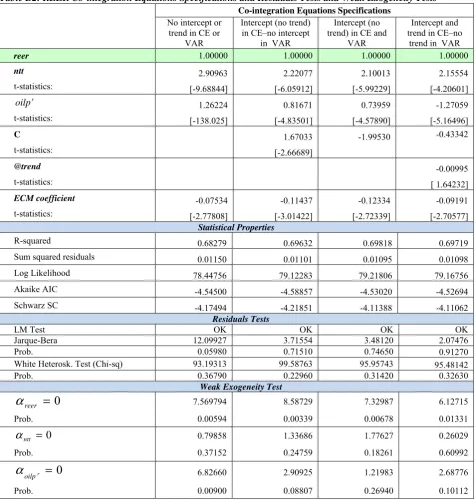
Then I perform Co-integration Test based on this VAR and as shown from the Table B1 in Appendix B both
Trace and Max-Eig Tests indicate existence of one co-integration relation between variables in four of
Co-integration Test Specifications. Since there are four competing versions I should choose more relevant one
among them. I estimate VECM in each of these four specifications and compare them with their properties.
The results are given Table B 2 in Appendix B. As shown from the Table B 2 fourth specification, i.e.
“Intercept and trend in CE–no trend in VAR” is not relevant one due to trend coefficient is not statistically
significant. The first specification also is not appropriate because of weak exogeneity test of real oil price is
not satisfactory here. Thus, I should choose relevant one among the second and the third specifications. One
can prefer rather the third specification than second in terms of R-squared, Sum squared of residuals, Log
Likelihood and highly significance of weak exogeneity Test. Thus, at the final I consider that the third
specification is the most relevant one. So, long-run relationship between real effective exchange rate, real oil
price and relative productivity derived from Johansen co-integration approach in given Equation (15)
reer
=
2
,
00
+
0
,
74
oilp
r+
2
,
10
ntt
(15)Note that this long-run equation is satisfactory in terms of autocorrelation, normality and heteroskedasticity tests
of residuals (See: Table B2 in Appendix B).
By using long-run coefficients of variables in Equation (15) I construct error correction term. ECM based on
Johansen approach is as below:
t t r t r t t t t
Q
dum
oilp
oilp
ntt
reer
ecm
reer
1
07
05
,
0
08
,
0
14
,
0
25
,
0
21
,
0
15
,
0
2 1 2 1+
Δ
+
Δ
−
−
Δ
+
Δ
+
−
=
Δ
− − − − (16)Since coefficient of error correction term is statistically significant and with negative sign I can conclude that
there is stabile long-run relationship between variables (See: Table B2, in Appendix B). Based on these error
correction terms I can calculate half-life speed (HLS) of adjustments towards long-run equilibrium (i.e. how
many quarter would need manat’s real effective exchange rate to restore half of its equilibrium) and it is
revealed that half-life speed of adjustments approximately takes 3-4 quarters in the case of Azerbaijani real
17
Interpretations of Estimation Results
Long-run coefficients derived from ARDL and Johansen approaches are very close to each-other as shown
from Equation (14) Equation (15) respectively. According to these equation one percent increase (decrease)
in real oil price leads to approximately 0.7 percent appreciation (depreciation) of real effective exchange
rate of manat. It is worth to note that this finding is in consistent with my research expectation and in line
with findings in case of other oil-exporting countries. For example Cashin (2002) for 22 commodity
exporting countries, Koranchelian (2005) for Algeria, Zalduendo (2006) for Venesuela, Issa et al. (2006) for
Canada, Habib and Kalamova (2007) for Norway, Saudi Arabia and Russia, Oomes and Kalcheva (2007) for
Russia, Jahan-Parvar and Mohammadi (2008) for 14 oil-exporting countries, Korhonen and Juurikkala (2009) for
9 OPEC countries. This finding has at least two important implications: the first one is that it supports the
existence of a co-integration between real oil prices and real exchange rates, and the Dutch Disease
hypothesis. Second one is that it indicates direction on causality, from real-oil price to real exchange rate.
It is important to note that we cannot conclude that Azerbaijani economy has contracted Dutch Disease just by
estimating impact of real oil prices on real exchange rates and in this regard we have to check all symptoms of
Dutch Disease in parallel with carefully testing alternative explanations of the observed processes.
One percent rise (decrease) in relative productivity causes approximately 2 percent appreciations (depreciations)
in real effective exchange rate of manat. This finding is also in line with my expectation and findings of other
studies. For example, statistically significant and positive impact of relative productivity, i.e. Balassa-Samuelson
Effect on real exchange rate also found by Halpern and Wyplosz (1997) for Transition countries of Eastern
Europe and Former USSR; Egert and Lommatzsch (2004) for Transition countries of Eastern Europe; Egert
(2005) for Bulgaria, Croatia, Romania, Russia, Ukraine, Turkey; Koranchelian (2005) for Algeria; Egert et al.
(2007) for Central and Eastern European economies; Habib and Kalamova (2007) for Russia; Zalduendo (2006)
for Venesuela; Oomes and Kalcheva (2007) for Russia and Korhonen and Juurikkala (2009) for 9 OPEC
countries. However, we should be careful when we interpret relative productivity in case of Azerbaijan. The point
is that increase in relative price of non-tradable is not sourced from productivity increase in tradable sector (i.e. in
manufacturing and agriculture) as states Balassa-Samuelson Hypothesis. If we look at the productivity growth in
tradable sector (manufacturing and agriculture) we can observe that there is downward trend here and on another
Figure C1-C2 in Appendix C). Therefore, increasing in relative price of non-tradable can be explained by rather
spending of oil revenues in non-tradable sector as budget expenditure than Balassa-Samuelson Effect. Indeed
main part of oil revenues in form of government expenditure is oriented to non-oil sector of economy and this
excess demand creates price increase in this sector (See: Figure C3-C4 in Appendix C). Thereby one can conclude
that increasing in relative price of non-tradable, one of the main determinants of appreciation of real effective
exchange rate mostly associates with high fiscal expansion, than Balassa-Samuelson Effect.
Study also reveals that according to coefficients of error correction terms derived from Johansen and ARDL
approaches 15-20 percent of short-run disequilibrium can be corrected toward long-run equilibrium path
within a quarter and half-life speed of adjustment approximately takes 3-4 quarters in the case of Azerbaijani
real effective exchange rate.
Conclusion and Policy Suggestions
Study reveals that real oil price has statistically significant and positive effect on Azerbaijani real effective
exchange rate which is similar to the experience of other oil-exporting countries. This finding provides us two
kinds of conclusion: The first is that it supports significant role of oil price in formation of equilibrium path of
real exchange rate of manat, therefore, Dutch Disease hypothesis. Second one is that it indicates direction on
causality, from real-oil price to real exchange rate.
It is important to note that we cannot conclude that Azerbaijani economy has contracted Dutch Disease just
by estimating impact of real oil prices on real exchange rates and in this regard we have to check all
symptoms of Dutch Disease in parallel with carefully testing alternative explanations of observed processes.
Study also finds statistically significant and positive impact of relative prices on real exchange rate of manat
which mostly associates with fiscal expansion than Balassa-Samuelson effect.
Since both of these determinants are tightly related to high fiscal expansion my policy suggestions mainly
focused on rather fiscal policy implementations than monetary policy issues. I think that all these challenges
particularly appreciation of real exchange rate which undermines competitiveness of economy mainly related to
management of oil revenues that is mainly fiscal issue than monetary. The main point is that when government
19
faces appreciation pressure. This is one of the potential channels of real exchange rate appreciation. Then
government spends these revenues mainly orienting into non-tradable sectors. This spending creates excess
demand for non-tradable goods which causes increasing in relative price of non-tradable. That is the second
potential channel of real exchange rate appreciation. Note that the second channel is more crucial than first one
because of nominal appreciation of manat somehow is prevented by Central Bank of Azerbaijan.
I would suggest that in parallel with such kind of spending (expensive reconstruction works on administrative
buildings, roads and bridges, construction of new buildings and etc.) government also should pay more
attention to development of non-oil tradable sector (manufacture and agriculture) which can help diversification
and sustainable development of economy. In this regard policy makers should focus on implementation of
policy measures that cover issues below:
- Efficiently using oil revenues in favor of non-oil tradable sector developing;
- Establishment and support of domestic industries;
- Involving foreign direct investments into non-oil tradable sector, especially export oriented branches;
- Promotions (tax concessions, subsidies, soft line credits and etc) to non-oil industry and agriculture,
especially to the export oriented and import substituting and also strategic branches;
- Elimination of institutional constraints, improvement of relevant legislation with a view to
developing non-oil tradable sector;
- Development of education and investment in human capital.
Reference
Alan, G. (1988). Oil windfalls: Blessing or curse? Oxford University Press, for the World Bank, New York, etc.
pp. 357.
Algozhina, A. (2006 ). Inflation Consequences of “Dutch Disease in Kazakhstan: The Case of Prudent Fiscal Policy”.
AlShehabi, O. and S. Ding (2008). Estimating Equilibrium Exchange Rates for Armenia and Georgia. IMF Working Paper, Middle East and Central Asia Department.
Bagirov, S. (2006). Azerbaijan’s oil revenues: ways of reducing the risk of ineffective use.
Central European University, Center For Policy Studies, Policy paper.
Buiter, W. and D. Purvis (1983). Oil, Disinflation and Export Competitiveness: A Model of the Dutch Disease.
National Bureau of Economic Research Working Paper 592 (Cambridge, Mass: NBER).
Borko, T. (2007) . The suspicion of Dutch disease in Russia and the ability of the government to counteract”
ICEG European Center. Working Paper Nr. 35.
Bruno, M. and J. Sachs (1982). Energy and Resource Allocation: A Dynamic Model of the Dutch Disease.
Review of Economic Studies, 49 (5), 845-59.
Cashin, P., L. Céspedes, and R. Sahay (2002). Keynes, Cocoa, and Copper: In Search of Commodity Currencies. IMF Working Paper 02/223 (Washington: International Monetary Fund).Clark, P.B. and MacDonald, R. (1998), “Exchange Rates and Economic Fundamentals: “A Methodological Comparison of BEERs and FEERs” IMF Working Paper No. WP/98/67.
Clark, P.B. and R.MacDonald (2000). Filtering the BEER: A Permanent and Transitory Decomposition. IMF Working Paper No. 00/144.
Corden, W.M., (1984). Booming Sector and Dutch Disease Economics: Survey and Consolidation. Oxford Economic Papers 36, 359-380.
Corden, W.M. and J.P.Neary (1982). Booming Sector and De-Industrialization in a Small Open Economy.
Economic Journal 92, 825-848.
Delechat, C. and M. Gaertner, (2008). Exchange Rate Assessment in a Resource-Dependent Economy: The Case of Botswana. IMF Working Paper WP/08/83.
Dickey, D. and W.Fuller (1981). Likelihood Ratio Statistics for Autoregressive Time Series with a Unit Root. Econometrica, Vol. 49.
Dobrynskaya, V. (2008). The monetary and exchange rate policy of the central bank of Russia under asymmetrical price rigidity. Journal of innovations economics.
Edwards, S. (1985). A commodity export boom and the real exchange rate: the money-inflation link. NBER Working Paper Series, Working Paper No. 1741.
Egert, B. (2009). Dutch disease in former Soviet Union: Witch-hunting? BOFIT Discussion Papers 4. Egert, B. (2005). Equilibrium exchange rates in Southeastern Europe, Russia, Ukraine and Turkey: Healthy or (Dutch) diseased? BOFIT Discussion Papers 3.
Egert, B. and C.S. Leonard (2007). Dutch Disease Scare in Kazakhstan: Is it real? William Davidson Institute Working Paper Number 866.
Egert, B. (2005). Equilibrium Exchange Rates in Southeastern Europe, Russia, Ukraine and Turkey: Healthy or (Dutch) Diseased? William Davidson Institute Working Paper. Number 770.
Egert, B. and K. Lommatzsch (2004). Equilibrium Exchange Rates in the Transition: The Tradable Price-Based Real Appreciation and Estimation Uncertainty. William Davidson Institute Working Paper Number 676.
Egert, B. and K. Lommatzsch and A. Lahrèche-Révil (2007). Real Exchange Rates in Small Open OECD and Transition Economies: Comparing Apples with Oranges? William Davidson Institute Working Paper
Number 859.
Enders, K. and H.Herberg (1983). The Dutch Disease: Causes, Consequences, Cure and Calmatives.
Welwirtschaftliches Archiv 119, 3, 473-9.
Enders, W. (2004). Applied Econometrics Time Series. University of Alabama, second edition.
Engle, R.F. and C.W.J. Granger (1987). Co-Integration and Error Correction: Representation, Estimation, and Testing. Econometrica,Vol.55,No.2., pp. 251-276.
Esanov, A., M. Raiser and W. Buiter (2001). Nature’s blessing or nature’s curse: the political economy of transition in resource-based economies. European Bank for reconstruction and development, working paper # 66.
E-Views 5 User’s Guide (2004) Quantitative Micro Software, USA.
21
Staff papers, Vol. 42, pp. 80-107.
Fatai, K. and L. Oxley and F.G. Scrimgeour (2003). Modeling and Forecasting the demand for Electricity in New Zealand: A Comparison of Alternative Approaches. The Energy Journal, vol. 24, pp. 75–102.
Gahramanov, E. and F. Liang-Shing (2002). The Dutch Disease in Caspian Region: the Case of Azerbaijan Republic. Economic Studies: Volume 5, 10.
Habib, M. and M. Kalamova (December 2007). Are there oil currencies? The real exchange rate of oil exporting countries. European Central Bank, Working Paper Series No 839.
Halpern, L. and C. Wyplosz (1997). Equilibrium Exchange Rates in Transition Economies. Staff Papers - International Monetary Fund, Vol. 44, No. 4, pp. 430-461.
Hasanli, Y. and R. Hasanov (2002). Application of Mathematical Methods in Economic Research. (in Azerbaijani), Baku.
Hasanov, F. (2004). Modeling of the interrelation between economic growth and inflation in the Azerbaijan Republic. Economic sciences: theory and practice. Azerbaijan State Economic University. (in Azerbaijani)
№3-4, p. 218-226.
IMF (2007). The Role of Fiscal Institutions in Managing the Oil Revenue Boom. International Monetary Fund, Washington DC.
Issa, R. and R. Lafrance, and J.Murray, (2006). The Turning Black Tide: Energy Prices and the Canadian Dollar. Working Paper 2006-29, Bank of Canada, Ottawa.
Jahan-Parvar, M. and H. Mohammadi (2008). Oil Prices and Real Exchange Rates in Oil-Exporting Countries: A Bounds Testing Approach. Illinois State University, Normal, East Carolina University, 28. Johansen, S. (1995). Likelihood-based inference in cointegrated vector auto-regressive models. Oxford University Press.
Johansen, S. (1988). Statistical analysis of cointegration vectors. Journal of Economic Dynamics and Control 12, 231-254.
Johansen, S. (2002). A small sample correction for the test of co-integrating rank in the vector autoregressive model. Econometrica 70, p. 1929-1961.
Johansen, S. and K.Juselius (1990). Maximum likelihood estimation and inference on cointegration with applications to the demand for money. Oxford Bulletin of Economics and Statistics 52, p.169-210.
Juselius, K. (2006). The cointegrated VAR model: methodology and applications. Oxford University Press Inc. Kalyuzhnova, Y. and M.Kaser (2006). Prudential Management of Hydrocarbon Revenues. Post-Communist Economies. Vol. 18, No. 2.
Krause, J. and M. Lücke (2005). Political and economic challenges of resource-based development in Kazakhstan and Azerbaijan. Institute of Political Science, Kiel University.
Koeda, J. and V. Kramarenko (2008). Impact of Government Expenditure on Growth: The Case of Azerbaijan. IMF Working Paper, Middle East and Central Asia Department.
Korhonen, I. and T. Juurikkala (2007). Equilibrium exchange rates in oil-dependent countries. BOFIT Discussion Papers No. 8.
Korhonen, I. and T. Juurikkala (2009). Equilibrium Exchange Rates in Oil Exporting Countries. Journal of Economics and Finance 33 (1), p.71-79.
Koranchelian, T. (2005). The equilibrium real exchange rate in a commodity exporting country: Algeria’s experience. IMF Working Paper 05/135, Washington D.C.
Kronenberg, T. (2004).The curse of natural resources in the transition economies. Economics of Transition 12(3). p. 399–426.
MacDonald, R. (1997). What determines real exchange rates: The long and short of it. IMF Working paper
97/21.
Mohammadi, H. and M. Jahan-Parvar (2009). Oil Prices and Exchange Rates in Oil-Exporting Countries: Evidence from TAR and M-TAR Models. Illinois State University, Normal, East Carolina University.
Muhammad, A. and R. Kashif (2010). Time Series Analysis of Real Effective Exchange Rates on Trade Balance in Pakistan. Journal of Yasar University 18(5) p. 3038-3044.
Narayan, P. K. (2005b). The structure of tourist expenditure in Fiji: evidence from unit root structural break tests. Applied Economics, 37, 1157–61.
Narayan, P. K. (2005). The saving and investment nexus for China: evidence from co-integration tests.
Applied Economics, 37, p.1979-1990.
Ollus, S. and S. Barisitz (2007). The Russian Non-Fuel Sector: Signs of Dutch Disease? Evidence from EU-25 Import Competition. BOFIT Online No. 2, Bank of Finland.
Oomes, N. and K. Kalcheva (2007). Diagnosing Dutch Disease: Does Russia Have the Symptoms. BOFIT Discussion Paper No 6.
Oteng-Abayie, E. and J. Frimpong (2006). Bounds Testing Approach to Cointegration: An Examination of Foreign Direct Investment Trade and Growth Relationships. American Journal of Applied Sciences 3 (11): 2079-2085, 2006, p.1546-9239.
Pesaran, H. M. and B. Pesaran (1997). Microfit 4.0. Oxford University Press, Oxford.
Pesaran, M. Hashem and Y. Shin (1997). An Autoregressive Distributed Lag Modelling Approach to Cointegration Analysis. Trinity College, Cambridge, England Department of Applied Economics, University of Cambridge, England First Version.
Pesaran, M.H., Y. Shin, and R.J. Smith (2001). Bound Testing Approaches to the Analysis of Level Relationships. Journal of Applied Econometrics, 16:289-326.
Phillips, P.C.B. and P. Perron (1988). Testing for a Unit Root in Time Series Regression”, Biometrika, Vol. 75, p.335-46.
Rautava, J. (2002). The role of oil prices and the real exchange rate in Russia’s economy. BOFIT Discussion Papers, No. 3.
Reza, Y. and S. Ramkishen (2006). Models of Equilibrium Real Exchange Rates Revisited: A Selective Review of the Literature. Centre for International Economic Studies Discussion Paper No. 0604, University of Adelaide, Australia.
Rosenberg, C.B. and T.O. Saavalainen (1998). How to Deal with Azerbaijan’s Oil Boom? Policy Strategies in a Resource-Rich Transition Economy. IMF Working Paper 98/6.
Sachs, J.D. and A.M. Warner (1997). Natural Resource Abundance And Economic Growth. Center for International Development and Harvard Institute for International Development .Harvard University Cambridge MA.
Stein, J.L. (1999). The evolution of the real value of the U.S.Dollar relative to the G7 currencies. Chapter 3 in Ronald MacDonald and J.L.Stein (eds.), Equilibrium exchange rates, Kluwer Academic Publishers, London, U.K. Sturm, M. and G. François and G. Juan (2009). Fiscal policy challenges in oil-exporting countries a review of key issues. European central bank, occasional paper series no 104.
Wakeman-Linn and P. Mathieu and B. Selm (2002). Oil funds and revenue management in transition economies: the cases of Azerbaijan and Kazakhstan.
Wijnbergen, S.V. (1984). Inflation, Employment, and the Dutch Disease in Oil-Exporting Countries: A Short-Run Disequilibrium Analysis. The Quarterly Journal of Economics, Vol. 99, No. 2 pp. 233-250. Zalduendo, J. (2006). Determinants of Venezuela’s equilibrium real exchange rate. IMF Working Paper
06/74, Washington D.C.
Appendix
[image:26.595.54.530.115.215.2]Appendix A: Estimation Outputs of ARDL Approach
Table A1: ADF and PP Unit Root Test Results
İn the level İn the first difference
Variables Test
Method Constant Trend Actual value Constant Trend Actual value
ADF Yes Yes -0.264032 No No -4.800968***
LOG(REER)
PP Yes Yes -0.416001 No No -5.038039***
ADF Yes Yes -2.398926 No No -5.549716***
LOG(OILP r) PP Yes Yes -2.398926 No No -5.601480***
ADF No No -2.041835 No No -6.571813***
LOG(NTT)
PP No No -2.018383 No No -6.720613***
[image:26.595.59.384.260.486.2]Note that *, ** and *** asateriks above actual values indicate statistical significance of actual value at the 1%, 5% and 10% significance levels respectively. Number of observations are 31. Seven lags were used in ADF test automatically and appropriate lag length is selected by Schwarz criterion
Table A2: Final ECM Specification with legged level variables Dependent Variable: DLOG(REER)
Method: Least Squares
Independent Variables Coefficient Std. Error t-Statistic Prob.
LOG(REER(-1)) -0.201001 0.052328 -3.841163 0.0008
LOG(NTT(-1)) 0.389387 0.099174 3.926307 0.0007
LOG(OILP r(-1)) 0.147203 0.026386 5.578826 0.0000
C 0.405052 0.221021 1.832639 0.0798
DLOG(NTT) 0.288799 0.081645 3.537239 0.0018
DLOG(NTT(-1)) -0.146740 0.080938 -1.813003 0.0829
DLOG(OILP r(-1)) -0.144408 0.036001 -4.011182 0.0005
DUM07Q1 0.056480 0.022799 2.477245 0.0210
R-squared 0.756533 Mean dependent var -0.003850
Adjusted R-squared 0.682435 S.D. dependent var 0.034770
S.E. of regression 0.019594 Akaike info criterion -4.809577
Sum squared resid 0.008830 Schwarz criterion -4.439516
Log likelihood 82.54844 Hannan-Quinn criter. -4.688946
F-statistic 10.20983 Durbin-Watson stat 2.010402
Prob(F-statistic) 0.000009
Appendix B. Estimation Outputs of Johansen Approach
Table B1: VAR Co-integration Test Output
Series: LOG(REER_T_04) LOG(NTT) LOG(OILP r)
Exogenous series: DUM07Q1 Lags interval: 1 to 2
Selected (0.05 level*) Number of Cointegrating Relations by Model
Data Trend: None None Linear Linear Quadratic
Test Type No Intercept Intercept Intercept Intercept Intercept
No Trend No Trend No Trend Trend Trend
Trace 1 1 1 1 2
Max-Eig 1 1 1 1 2
*Critical values based on MacKinnon-Haug-Michelis (1999)
[image:26.595.57.421.567.694.2]Table B2: REER Co-integration Equations Specifications and Residuals Tests and Weak Exogeneity Tests
Co-integration Equations Specifications
No intercept or trend in CE or
VAR
Intercept (no trend) in CE–no intercept
in VAR
Intercept (no trend) in CE and
VAR
Intercept and trend in CE–no
trend in VAR
reer 1.00000 1.00000 1.00000 1.00000
ntt 2.90963 2.22077 2.10013 2.15554
t-statistics: [-9.68844] [-6.05912] [-5.99229] [-4.20601]
r
oilp 1.26224 0.81671 0.73959 -1.27059
t-statistics: [-138.025] [-4.83501] [-4.57890] [-5.16496]
C 1.67033 -1.99530 -0.43342
t-statistics: [-2.66689]
@trend -0.00995
t-statistics: [ 1.64232]
ECM coefficient -0.07534 -0.11437 -0.12334 -0.09191
t-statistics: [-2.77808] [-3.01422] [-2.72339] [-2.70577]
Statistical Properties
R-squared 0.68279 0.69632 0.69818 0.69719
Sum squared residuals 0.01150 0.01101 0.01095 0.01098
Log Likelihood 78.44756 79.12283 79.21806 79.16756
Akaike AIC -4.54500 -4.58857 -4.53020 -4.52694
Schwarz SC -4.17494 -4.21851 -4.11388 -4.11062
Residuals Tests
LM Test OK OK OK OK
Jarque-Bera 12.09927 3.71554 3.48120 2.07476
Prob. 0.05980 0.71510 0.74650 0.91270
White Heterosk. Test (Chi-sq) 93.19313 99.58763 95.95743 95.48142
Prob. 0.36790 0.22960 0.31420 0.32630
Weak Exogeneity Test
0
=
reer
α
7.569794 8.58729 7.32987 6.12715Prob. 0.00594 0.00339 0.00678 0.01331
0 =
ntt
α 0.79858 1.33686 1.77627 0.26029
Prob. 0.37152 0.24759 0.18261 0.60992
0
=
r
oilp
α
6.82660 2.90925 1.21983 2.68776Appendix C: Graphic Illustrations
Figure C1: Productivity growth in non-oil tradable sector, %
Source: Author’s own calculation based on SSCAR data.
Figure C2: ULC growth by sectors, %
Source: Author’s own calculation based on SSCAR data.
[image:28.595.110.487.463.716.2]Figure C3: Government expenditures and government investments to non-oil tradable and non-tradable sectors
a) Government Expediture Growth b) Government investments, million AZN
Source: Author’s own calculation based on SSCAR data.
Figure C4: Tradable and non-tradable prices
[image:29.595.111.488.385.636.2]