Energetic Extended Edge Finding Filtering Algorithm for Cumulative Resource Constraints

http://dx.doi.org/10.4236/ajor.2013.36056

Energetic Extended Edge Finding Filtering Algorithm for

Cumulative Resource Constraints

Roger Kameugne1,2, Sévérine Betmbe Fetgo3, Laure Pauline Fotso3

1_{Department of Mathematics, Higher Teachers’ Training College, University of Maroua, Maroua, Cameroon} 2_{Department of Mathematics, Faculty of Sciences, University of Yaounde I, Yaoundé, Cameroon} 3_{Department of Computer Sciences, Faculty of Sciences, University of Yaounde I, Yaoundé, Cameroon}

Email: [email protected], [email protected], [email protected], [email protected]

Received September 28, 2013; revised October 28, 2013; accepted November 5, 2013

Copyright © 2013 Roger Kameugne et al. This is an open access article distributed under the Creative Commons Attribution License, which permits unrestricted use, distribution, and reproduction in any medium, provided the original work is properly cited.

ABSTRACT

Edge-finding and energetic reasoning are well known filtering rules used in constraint based disjunctive and cumulative scheduling during the propagation of the resource constraint. In practice, however, edge-finding is most used (because it has a low running time complexity) than the energetic reasoning which needs

 

2

n

 time-intervals to be considered (where n is the number of tasks). In order to reduce the number of time-intervals in the energetic reasoning, the maxi-

mum density and the minimum slack notions are used as criteria to select the time-intervals. The paper proposes a new filtering algorithm for cumulative resource constraint, titled energetic extended edge finder of complexity

 

3

n  . The new algorithm is a hybridization of extended edge-finding and energetic reasoning: more powerful than the extended edge-finding and faster than the energetic reasoning. It is proven that the new algorithm subsumes the extended edge-finding algorithm. Results on Resource Constrained Project Scheduling Problems (RCPSP) from BL set and PSPLib librairies are reported. These results show that in practice the new algorithm is a good trade-off between the filtering power and the running time on instances where the number of tasks is less than 30.

Keywords: Constraint-Based Scheduling; Global Constraint; Cumulative Resource; Energetic Reasoning;

Edge-Finding; Extended Edge-Finding; Maximum Density; Minimum Slack

1. Introduction

Scheduling is the process of assigning resources to tasks or activities over the time. There exist many types of scheduling problems following the tasks properties (pre- emptive or non-preemptive), the type of resources (dis- junctive or cumulative) and the objective function (make- span, time late...). When a unique cumulative resource with non-preemptive tasks is considered, the problem is called cumulative scheduling problem (CuSP).

In a CuSP, a set of tasks T has to be executed on a

resource of fixed capacity C. Each task i requires a

fixed and constant amount of resource ci, and has to be executed during a fixed amount of time pi without in- terruption between an earliest start time esti (release date) and a latest completion time lcti (deadline). A solution of a CuSP instance is an assignment of valid start time si to each task i in such a way that resource constraints are satisfied i.e.,

: esti i i i lcti

i T s s p

      (1)

,

:

i i i i i T s s p

c C

 

   





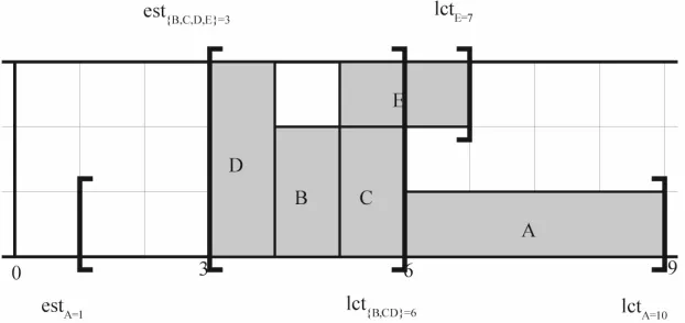
 (2)

The inequalities in (1) ensure that each task is assigned a feasible start and end time, while (2) enforces the re- source constraint. An example of CuSP is given in

Figure 1.

The energy of a task i, is defined as e_i c_i p_i, its

earliest completion time as ecti estipi and its latest start time as lstilctipi. The energy notation along with that of earliest start and latest completion time may be extended to non-empty sets of tasks as follows:

, est min est , lct max lct

j j j

j j

j

e_ e _{ }

 







  (3)

where  is a non-empty set of tasks. By convention, if

 is the empty set, est , lct , and

0

[image:2.595.143.454.87.234.2]

Figure 1. A scheduling problem of 5 tasks sharing a resource of capacity C = 3.

task iT , est_ip_ilct_i and c_i C, otherwise the

problem has no solution.

The CuSP is a NP-complete problem [1]. Therefore, only relaxation of the problem, for which it is possible to implement a polynomial time algorithm exists. In [2], the cumulative resource constraint is modelized by the global constraint CUMULATIVE in a constraint programming approach. The global constraint CUMULATIVE embeds many filtering algorithms. Among these algorithms, en- ergetic reasoning, edge-finding and timetabling are the most used.

1.1. Related Works

To our knowledge, the word “energetic edge-finder” was firstly used in [3] where the author incorporates the en- ergy-based deduction rule to edge-finder algorithm for disjunctive (unary) resource. The idea of hybridization of the edge-finding rule and the energetic reasoning for cumulative resource was suggested in [4]. Indeed, in [4], Mercier and Van Hentenryck propose a two phase edge-finding algorithm where in the first phase, the po- tential adjustment values are computed. They found that many of these potential update values are unused and can be used inside an energetic-based second phase. After this suggestion, many filtering algorithms, hybridization of edge-finding rule and energetic reasoning have been proposed [5,6]. In [6], the authors use in the first phase, the edge-finding algorithm of [7,8] to compute the poten- tial update values and identify the corresponding time bounds of task intervals which provide the maximum update values. To each task, the time bounds used in the second phase is either the task intervals of maximum density or the task intervals of minimum slack. The re- sulting algorithm runs in

 

2

n

 since both phases have this complexity. This algorithm was later improved in [5] by choosing for each task, the time bounds of task inter- vals of both maximum density and minimum slack which provide the maximum update values. Experimental re- sults on RCPSP of the PSPLib [9] library and BL set [10]

show that this variant is a good trade-off between the filtering power and the complexity but it does not domi- nate the edge-finding algorithm.

Energetic reasoning is one of the most powerful filter- ing algorithm in cumulative scheduling problems [1,10] since it dominates all the other rules (edge-finding [4,7, 8,21], extended edge-finding [4,11], timetable [1], time- table edge-finding [12], timetable extended edge-finding [13]) except the not-first/not-last rule [14,15]. However, it is not commonly used because it has a high running time (

 

3

n

 time complexity), needs a high number of time-intervals to be considered and its success highly depends on the tightness of the variable bounds (highly cumulative problems). Recently, in [16], the authors pro- posed an approximative criterion for the potential of the energetic reasoning which allows the decrease of the running time with more nodes to explore in the search tree. The combination of a solver of the CP and SAT techniques for conflict analysis played recently an im- portant role to solve cumulative scheduling problems effi- ciently [17,18].

In this paper, it is extended the energetic edge finder of [5] by adding the guarantee that the final algorithm de- duces more than edge-finding and extended edge-finding. The main idea of our energetic extended edge finder is the combination of the best properties of (extended) edge-finding rule (interesting time bounds and good run-ning time) and energetic reasorun-ning (powerful filtering rule). The paper starts with the hypothesis that, the time bounds of task intervals used in the (extended) edge- finding algorithm can be interesting in an energetic rea- soning. Based on this hypothesis, the number of time intervals to be considered in an energetic reasoning is reduced to those of (extended) edge-finding.

1.2. Contribution

energetic reasoning. Indeed, in [7,8], a complete edge- finding algorithm is proposed based on maximum density and minimum slack. The minimum slack is used in [11] to perform the extended edge-finding algorithm. The algorithm presented in this paper is an energetic version of the edge-finding and the extended edge-finding algo- rithms of [7,8,11] respectively. The complexity of the corresponding algorithm is

 

3

n

 where n is the

number of tasks since each of the algorithm of [7,8] and [11] are quadratic.

It is obvious that the new algorithm subsumes the edge-finding and the extended edge-finding algorithms. The filtering power of this algorithm is less than the one of the energetic reasoning, but in practice, it is a good trade-off between the filtering power and the running time. Empirical evaluation of the algorithm on the RCPSP instances of well known library prove that, the new algorithm performs in most of the cases better in term of reduction of number of nodes of the search tree than the quadratic extended edge-finding [11], but needs more time to do so, for instances of more than 30 tasks.

The rest of the paper is organized as follows: Section 2 is devoted to the specification of the edge-finding rule and the energetic reasoning. In Section 3, the new ener- getic extended edge-finder is described and some of its properties are deduced. Experimental results are provided in the last Section.

2. Edge-Finding Rule and Energetic

Reasoning Rule

In this section, it is specified the (extended) edge-finding rule as well as the energetic reasoning.

2.1. Edge-Finding and Extended Edge-Finding Rules

Let T be the set of tasks of a CuSP. If the energy e

of a set of tasks  T is larger than the available en-

ergy C



lct_est_



, then the problem has no feasible solution. Overload checking algorithms typically enforce

the following relaxation of this feasibility condition, which may be computed in 



nlogn



time [19,20].

Definition 1 (E-Feasibility) ([4]) A CuSP problem is E-feasible if:





, , lct est .

T C _{ } e_

       (4)

For a given CuSP, an edge-finding rule identifies a set of tasks  T and a task i  such that, in any so-

lution, all tasks of  end before the end of i. More

precisely, if the scheduling of task i as early as possi-

ble (i.e., starting at esti) induces an overload in the in- terval



est , lct 



then, all the tasks in  end before the end of i noted here i as in [21]. When all

tasks of a set  end before the end of a task i, then

the release date of task i is updated to:





1

esti est rest , i i

i c

c 

 

   _  _

 

 (5)

for all    such that rest



,ci



0,









lct est



if

rest ,

0 otherwise

i i

e C c

c         

 _{ }

 (6)

Proposition 1 provides conditions under which all tasks of a set  of a CuSP end before the end of a task i.

Proposition 1 [4,7,8,11,21] Let  T be a set of tasks of a CuSP of capacity C and iT be a task.

 i



lct est  i



;

e_ C _ _  i (EF)

ectilct i; (EF1)









est est ect

. ect est lct est

i i

i i

i

e c C



   

 



 

    

  (EEF)

And if i then the earliest start time of task i is

updated to

 





rest , 0

1 est max est , max est rest ,

i

i i i

i c

c c

 

 

 _{ }

 

 _  _

 _{ }

 

(Upd)

with











if

rest ,

0 otherwise

i i

e C c lct est

c         

 _{ }

 (7)

Rules (EF) and (EF1) are known as edge-finding de-tection rules while (EEF) is the extended edge-finding detection rule. It is proved in [4] that a complete edge-finding algorithm that only considers sets  T

and   , which are task intervals can be imple- mented. The definition of the task intervals is given in Definition 2.

Definition 2 (Task Intervals) (After [22]) Let j k, T. The task intervals j k, is the set of tasks





, est est lct lct .

j k s T j s s k

      (8) In [7,8], the authors propose a quadratic edge-finding algorithm based on maximum density and minimum slack notions.

Definition 3 [7,8] Let  be a task set of an E- feasible CuSP. The slack of the task set , denoted

SL_, is given by:



lct est



.

SL_ C _ _ e_

Definition 4 [7,8] Let i and k be two tasks of an E-feasible CuSP. 

 

k i, is a task depending on the tasks k and i, where est_{ }k i_, esti and that defines

such that estjesti,

 



lctk est k i,



 k i k, ,



lctk estj



j k, .

C  _ e_ C  e (9)

The detection of the classic edge-finding rule (EF) is done with the task intervals of minimum slack. For ad- justment, as it is proved in [7,8], the task intervals of minimum slack and the one of maximum density are considered.

Definition 5 [7,8] Let  be a task set of an E- feasible CuSP. The density of the task set , denoted

Dens_, is given by:

. lct est

e

Dens_ 

 

 

Definition 6 [7,8] Let i , k be two tasks of an E-feasible CuSP. 

 

k i, is a task depending on the tasks k and i, where estiest_{ }k i_, and that defines

the task intervals with the maximum density: for all tasks jT such that estiestj,

 

 

, , ,

,

. lct est lct est

k i k j k

k j k k i

e

e _

  



  (10)

The main idea of the edge-finding algorithm of [7,8] is that once the relation i is discovered, then it is not

necessary to iterate over all subsets  of . It is enough to consider only (1) subset with minimum slack and estesti and (2) subset with maximum density and est esti. Using those two subsets, if esti can be improved, then it will be updated, although not necessar- ily immediately to the best value. More iterations of the algorithm may be needed for that.

The extended edge-finding rule (EEF) detects addi- tional updates missing by the edge-finding rule. In [11], the authors propose a quadratic extended edge-finding algorithm based on minimum slack notion. This algo- rithm supposes that the fix point of the edge-finding is reached and looks for the upper bound of the task inter- vals of minimal slack instead of the lower bound as it is the case for the edge-finding algorithm.

Definition 7 [11] Let i and j be two tasks of an E-feasible CuSP with estiestj. 

 

j i, is a task de-

pending on the tasks j and i, where lct_{ }j i_, lcti

and that defines the largest task intervals with the mini- mum slack: for all kT such that lctk lcti

 



lct j i, estj



j, j i,



lctk estj



j k, .

C _  e _ C  e (11)

2.2. Energetic Reasoning

In the edge-finding rule, the energy required by a non- empty set of tasks  only considers tasks which are completely processed within the time window



est , lct 



while, the partial contribution of each task is taken into

account in the energetic reasoning. There exists many varieties of energy consumption required by a task de- pending on the type of tasks, Fully Elastic energy and Partial Elastic energy for preemptive tasks and Left- shift/Right-shift energy for non-preemptive tasks [10].

Let i be a task and



a b,



be a time interval with ab. The left-shift/right-shift energy consumption re-

quired by i over



a b,



noted W a b i



, ,



is the non-

negative minimum of 1) the volume in the interval



a b,



, 2) the energy of task i, 3) the left shifted en-

ergy, and 4) the right shifted energy i.e.,













, ,

max 0, min , ,ect , lst

i i i i

W a b i

c b a p a b

     (12)

The overall energy consumption required by all tasks noted W a b

 

, over an interval



a b,



is defined as

 

,



, , .



i T

W a b W a b i







(13)

For a given CuSP, it is obvious that if there exists a time interval



a b,



with ab such that its overall

required energy consumption is more than available en- ergy, then the problem is infeasible. This necessary con- dition is provided in the following proposition.

Proposition 2 [1] Let



a b,



be a time interval with ab. If





 

,

C ba W a b (14)

then the problem is infeasible.

In [1,10], the authors give a precise characterization of time bounds for which the necessary condition of the existence of a feasible scheduling should be guaranteed. This necessary condition is more powerful than the E-feasible one defined earlier. There exist

 

2

n

 rele- vant intervals to be considered to detect infeasibility. These intervals correspond to start and completion times of tasks. If









 





1

2

: est ,ect ,lst ,

: lct ,ect ,lst

and : est lct i i i i T

i i i i T

i i i T

O

O

O t t





 



  







then the relevant intervals are given by

 

a b, O1O2,

for a fixed aO1:

 

a b,  O1 O a

 

, and for a fixed

2

bO :

 

a b, O b

 

O₂ , with ab. The authors

propose a quadratic algorithm for testing this necessary condition in [1,10].

The left-shift energy required of a task i over a time

interval



a b,



defined by

















, ,

min , , min ect , max est ,

l

i i i i

W a b i

c b a p b a

is ci times the number of time units during which i executes after time a if i is left-shifted, i.e., sche-

duled as soon as possible. If scheduling task i as early

as possible (i.e., starting at esti) induces an overload in the interval



a b,



then task i ends after b and esti can be updated according to Proposition 3.

Proposition 3 [1] Let



a b,



be an interval with ab and i be a task such that



a b,







est , ecti i



 . If

 

,



, ,



l



, ,







W a b W a b i W a b i   C b a (ER)

holds, then the earliest start time of task i is updated to:

 







 







est max est ,

1 _{, , , .}

i i

i i

a

W a b W a b i C c b a

c   

 



 

      _{ }

  

(ERupd)

No specific characterization of relevant intervals for the adjustment was proposed so far. With the

 

2

n



relevant intervals used for infeasibility test, it is derived a

 

3

n

 algorithm for adjustment in [1,10]. In practice, the energetic reasoning adjustment is too time-consum- ing for producing any useful result [1]. The paper tries to determine a better trade off between the filtering power and running time by reducing the number of intervals to examine. It is used the time bounds of task intervals of edge-finding and extended edge-finding algorithm in an energetic reasoning. The corresponding algorithm runs in

 

3 n

 as pure energetic reasoning adjustment.

3. The Energetic Extended Edge-Finder

3.1. The Rule

The energetic extended edge-finding rule is obtained by substituting e_ by W



est ,lct_{ }



in the edge-finding

detection rule (EF) and the extended edge-finding detec- tion rule (EEF). It can be observed that the energetic reasoning rule (ER) is a generalization of rules (EF) and (EEF) with more strong energy consumption required by tasks over interval



est ,lct . 



The energetic extended edge-finding combines the techniques of edge-finding, extended edge-finding and partially the energetic rea- soning. The new adjustment rule is obtained by substi- tuting the energy e_ by W



est ,lct_{ }



in the (ex-

tended) edge-finding adjustment rule.

3.2. Algorithm

The algorithm proposed in this Section is an energetic version of the edge-finding and the extended edge-find- ing algorithm of [7,8,11] respectively. The time bounds

of task intervals used in the edge-finding (resp. the ex- tended edge-finding) for detection and adjustment are used in an energetic reasoning. The new algorithm runs in

 

3

n

 since each of the edge-finding and extended edge-finding algorithms are quadratic [7,8,11].

The algorithm is broken into two parts to make it more digest. The first part is an energetic variant of the edge- finding algorithm of [7,8] while the second part is the one of the extended edge-finding algorithm of [11] (ad- justments missing by the edge-finding and detect with the extended edge-finding).

3.2.1. First Part

This part consists only in adding an inner loop in the edge-finding algorithm of [7,8] after detection of time bounds, to recompute the energy of each task intervals

 plus the partial contribution of the rest of tasks .

T It is presented in Algorithm 1 where:

1) The first outer loop (line 3) selects, in the order of non-decreasing deadlines, the tasks kT which form

the possible upper bounds of the task intervals.

2) The first inner loop (line 5) selects the tasks iT

that includes the possible lower bounds for the task in- tervals, in non-increasing order by release date. If lctilctk, then the energy and density of i k, are cal-

culated; if the new density is higher than _{ }k i k, , where

the task 

 

k i, is specified in Definition 6, then

 

k i,

 becomes i (line 9). If lctilctk, then if the current 

 

k i, satisfies est_{ k i,} lct_k and ect_i

 ,

est_{k i}

 (line 12), then the energy required by interval

 ,



estk i ,lctk



 is computed in the inner loop of line 13.

The condition of line 15 checks if the interval

 ,



estk i ,lctk



 is overloaded (see inequality (12)) and if

the condition of line 17 is fulfilled, then the potential update Dupdi of the release date of i is calculated (line 18), based on the current interval est_{ }k i, , lctk



. This potential update is stored only if it is greater than the previous potential update value calculated for this task using the maximum density time bounds. The re- lease date of task i is updated at line 20 when the en-

ergetic reasoning condition of line 19 is fulfilled (see inequality (ER)).

3) The second inner loop (line 23) selects i in

non-decreasing order by release date. The energies stored in the previous loop (line 21) are used to compute the slack of the current interval i k, . If the slack is lower

than that of _{ k i k, ,} where 

 

k i, is specified in Definition 4, then 

 

k i, becomes i (see line 25). For

any task i with a deadline greater than lct_k, if the

Require: T is an array of tasks

Ensure: A lower bound esti is computed for the release date of each task 1 for i T do

2 esti:=est Dupdi, i:=,SLupdi:= 3 for kT by non-decreasing deadline do 4 Energy: 0, max Energy: 0, est:  5 for iT by non-increasing release dates do 6 if lctilctk then

7 Energy:=Energyei

8 if max k i k

Energy Energy lct est lct est

 



 

 _{ } 

  then

9 maxEnergy:Energy est, :esti 10 else

11 a:=est b, :=lct W a bk,  , := 0 12 if b>aectia then 13 for jT do

14 W a b , :=W a b , W a b j , ,  15 if C b a  <W a b ,  then 16 fail (No solution exists)

17 if W a b , W a b i , ,  Cci  b a> 0 then 18 := max ,   , , ,  i  

i i

i

W a b W a b i C c b a Dupd Dupd a

c

       



  

 _{ }

 

19 if W a b , W a b i , ,W a b il , , > C b a   then 20 esti:= maxest Dupdi, i

21 Ei:=Energy 22 minSL: , est:=lctk

23 for i T by non-decreasing release date do 24 if C lct kesti Ei minSL then 25 est:esti, minSL:C lct( kest)Ei 26 if lcti>lctk then

27 a:est b, :lct W a bk,  , : 0 28 if b>a then 

29 for jTdo

30 W a b , :W a b , W a b j , , 

31 if C b a  <W a b ,  then 32 fail (No solution exists)

33 if W a b , W a b i , , Cci  b a> 0 then 34 : max ,  , , ,  i  

i i

i

W a b W a b i C c b a SLupd SLupd a

c

       

 _  _

 

 

35 if W a b , W a b i , ,W a b il , , > C b a   then 36 esti: max est SLupd Dupdi, i, i

Algorithm 1. Energetic extended edge finding algorithm in 3

(n )

 time.

31 checks if the interval est_{ }k i_, , lctk



is overloaded (see inequality (12)). If the condition of line 33 is ful- filled, then the potential update SLupdi of the release date of i is calculated (line 34), based on the current

interval est_{ }k i_, ,lctk



. This potential update is stored

only if it is greater than the previous potential update value calculated for this task using the minimum slack time bounds. If the energetic reasoning condition is ful- filled at line 35 (see inequality (ER)), then the release date of task i is updated at line 36.

4) At the next iteration of this first outer loop, 

 

k i, and 

 

k i, are re-initialized.

This first algorithm (Algorithm 1) corresponds to the

energetic edge-finding algorithm.

3.2.2. Second Part

This part is the energetic version of the extended edge- finding algorithm of [11]. It consist in adding an inner loop in the extended edge-finding algorithm of [11] after detection of time bounds, to recompute the energy of each task intervals  plus the partial contribution of the rest of tasks T. The corresponding algorithm is presented in Algorithm 2 where:

1) The outer loop (line 37) iterates through the tasks

jT forming the possible lower bounds of the task

intervals.

2) The inner loop (line 39) selects the tasks iT that

comprise the possible upper bounds for the task intervals, in non-decreasing order of deadlines. If estjesti, then the energy and the slack of j i, are calculated. The

slack is then compared to the slack of _{j, j i,} (see line 42) where 

 

j i, is specified in Definition 7. If the new slack is higher, 

 

j i, becomes i (line 43). If

estj esti (line 44), then if the current 

 

j i, satisfies

37 for jT do

38 Energy: 0,max Energy: 0, lct:estj

39 for iT (T sorted by non-decreasing deadlines) do 40 if



estjesti



then

41 Energy:Energyei

42 if



C lct



iestj



EnergyC lct



estj



maxEnergy



then

43 maxEnergy:Energy lct, :lcti

44 else

45 a:est bj, :lct W a b,  , : 0

46 if b>aectia then

47 for kT do

48 W a b , :=W a b , W a b k , , 

49 if C b a<W a b ,  then 50 fail (No solution exists)

51 if W a b , W a b i , ,W a b il , , > C b a then

52 := max ,  ,  , ,  i   i i

i

W a b W a b i C c b a est est a

c

       

 _   _

 

 

53 for iT do 54 esti:=esti

Algorithm 2. Energetic extended edge finding algorithm in 3

(n )

 ,

lct j i estj and ecti estj(line 46), then the energy required by interval est ,lctj _{ }j i_,



is computed in the inner loop of line 47. The condition of line 49 checks if the interval est_{ }k i_, ,lctk



is overloaded (see inequality (12)). If the energetic reasoning condition is fulfilled at line 51 (see inequality (ER)), then the release date of task

i is updated at line 52 based on the current potential

update value determined by interval est ,lctj _{ }j i_,



. 3) At the next iteration of this outer loop, 

 

j i, is re-initialized.

Merging Algorithms 1 and 2, the corresponding algo-

rithm title “EnEEF” is an energetic extended edge-find- ing algorithm.

3.3. Some Properties of EnEEF

The energetic extended edge-finding algorithm EnEEF is compared to the conjunction of the edge-finding and the extended edge-finding. It is proved that, this algorithm subsumes the conjunction of edge-finding and extended edge-finding algorithm.

3.3.1. The Energetic Extended Edge-Finder EnEEF Performs Some Additional Adjustments Missing by (Extended) Edge-Finding

Using the CuSP instance of Figure 1, it is found that the

energetic extended edge-finder EnEEF performs addi- tional adjustments missing by (extended) edge-finding. Indeed, the application of the (extended) edge-finding algorithm on the CuSP instance of Figure 1 doesn’t

produce any adjustment whereas the application of our energetic extended edge finder EnEEF permits to update the release date of task A from 1 to 5. When the task B

(resp. C or D) is considered at the outer loop of line 3,

the bounds of the task intervals of maximum density are [3,6) and the condition of line 19 holds for a3 and

6.

b It follows that

 

















, , , , ,

8 2 10 9 3 6 3 l

W a b W a b A W a b A

C b a

 

         

and

 



 











, , ,

8 0 3 1 6 3 2. A

W a b W a b A  Cc b a

     

Therefore, the release date est_A is updated to

 

,



, ,

 





est

3 2 5.

A A

A

W a b W a b A C c b a

a

c

   

 

   

 

  

The reader can check that no propagation is performed by the timetable edge-finding rule of [12] and the timeta- ble extended edge-finding rule of [13] on the CuSP in- stance of Figure 1.

3.3.2. The Energetic Extended Edge-Finder EnEEF Subsumes the Edge-Finding Algorithm

Theorem 1 The energetic extended edge-finder EnEEF

subsumes the edge-finding algorithm of [7,8].

Proof. It is important to prove that the edge-finding algorithm can not propagate anything when the energetic extended edge-finder EnEEF reaches the fix point.

By contradiction: assume that the energetic extended edge-finder EnEEF reaches the fix point, and that how- ever, the edge-finding algorithm can propagate i.e., there

are i,  and ,    such that (EF) or (EF1)

holds and (Upd) improves esti using . It will be prove (by contradiction) that the energetic extended edge-finding algorithm EnEEF can update the time bounds of task i.

1) The rule (EF1) holds. In this case, two subcases are considered:

(a) If estesti, then the energy contribution of task

i in the time interval



est ,lct_{ }



is c_i



lct_est_i



since ecti lct . The inequality





1

est rest , i esti i

c c

   (16)

holds since the release date of task i is updated using

the rule (Upd) and it is algebraically equivalent to



lct est





lct est .



i i

e_c _ C _ _ (17)

Let kT be a task such that lctk:lct. According to [7,8],  is the task intervals of minimum slack (Definition 4) and it follows

 





 









, ,

,

lct est lct est

lct est .

k i k k k i

i i

C e C e

c 

    



    

  (18)

When the task k is considered in the outer loop of line

3, in the second inner loop of line 23 the condition

 

,



, ,



_l



, ,







W a b W a b i W a b i   C b a (19)

is detected at line 35 since

 





_{ }

, ,

, , ,

k i k

W a b W a b i e

 

 

and W a b il



, ,



ci



lctesti



where a: est  k i, and

: lctk

b  and the adjustment follows.

(b) If estiest, then the energy contribution of task

i in the time interval



est , lct_{ }



is c_i



lct_est_



since ecti lct . The inequality





rest ,ci 0 (20) holds since the release date of task i is updated using

the set  and the rule (Upd) and it is algebraically equivalent to



lct est





lct est .



i

e_c _ _ C _ _ (21)

(Definition 6) and it follows

 

 

, ,

,

. lct est lct est

k i k

i

k k i

e _e

C c





 _

 

  

  (22)

Therefore, it appears that

 k i k, , i



lctk est  k i,





lctk est  k i,



.

e_ c  _ C  _ (23)

When the task k is considered in the outer loop of line

3, in the first inner loop of line 5 the condition

 

,



, ,



l



, ,







W a b W a b i W a b i   C b a (24)

is detected at line 19 since

 





_{ }

, ,

, , ,

k i k

W a b W a b i e

 

 

and W a b il



, ,



ci



lctk est_{ }k i_,



where a: est  k i,

and b: lct k and the adjustment follows.

2) The rule (EF) holds: Let kT be a task such that

lct : lct .k   According to [7,8],  is the task intervals of minimum slack (Definition 4) and it follows

 



lctk est k i,



 k i k, , i.

C e e



 

   (25) When the task k is considered in the outer loop of line

3, in the second inner loop of line 23 the condition

 

,



, ,



_l



, ,







W a b W a b i W a b i   C b a (26)

is detected at line 35 since

 





_{ }

, ,

, , ,

k i k

W a b W a b i e

 

 

and W a b il



, ,



ei where a: est  k i, and b: lct k and the adjustment follows using the potential update values previously computed.■

According to this theorem, the first outer loop of line 3 ensures us that the fix point of the edge-finding rule will always be reached. This result is used to demonstrate that our algorithm dominates the extended edge-finding rule. In the following theorem, it is proved that, at the fix point of the edge-finding rule, if the extended edge-finding rule detects the relation i for a set of tasks  and a

task i then the set  can help to compute the poten-

tial updated value of esti.

3.3.3. The Energetic Extended Edge-Finder EnEEF Subsumes the Extended Edge-Finding Algorithm

Theorem 2 [11] Let  T be a set of tasks and iT be a task of an E-feasible CuSP. At the fix point of the edge-finding rule, if the extended edge- finding rule detects i then





1





rest , i 0 and est rest , i est .i i

c c

c 

 

  _  _

 

Using theorem 2, it is derived the following theorem:

Theorem 3 The energetic extended edge-finder EnEEF subsumes the extended edge-finding algorithm of [11].

Proof. As in Theorem 1, it is prove that the extended

edge-finding algorithm can not propagate anything when the energetic extended edge-finder EnEEF reaches the fix point.

The contradiction is used: assume that the energetic extended edge-finder EnEEF reaches the fix point, and that however, the extended edge-finding algorithm can propagate i.e., there are i,  and ,    such

that (EEF) holds and (Upd) improves esti using . It will be prove (by contradiction) that the energetic ex- tended edge-finding algorithm EnEEF can update the time bounds of task i.

Let jT be a task such that est : est ._j  _ Accord-

ing to [11],  is the task intervals of minimum slack (Definition 7) and it follows

 





 









, ,

,

lct est lct est

ect est .

j j i j

j i

i i

C e C e

c



    



    

  (27)

When the task j is considered in the outer loop of line

37, in the inner loop of line 39 the condition

 

,



, ,



l



, ,







W a b W a b i W a b i   C b a (28)

is detected at line 51 since

 





_{ }

, ,

, , ,

j j i

W a b W a b i e

 

 

and W a b il



, ,



ci



ectiest



where : esta j and

 ,

:

j i

b lct



 . According to Theorem 1, the fix point of

the edge-finding rule is reached and the Theorem 3 shows that the task intervals used for detection can also be used to perform the adjustment. Therefore, an adjust- ment is performed at line 52 since this adjustment is jus- tified by the condition of line 51.■

4. Experimental Results

For our experiments, it is consided the resource-con- strained project scheduling problems (RCPSP). A RCPSP consists of a set of resources of finite capacities, a set of tasks of given processing times, an acyclic network of precedence constraints between tasks, and a horizon (a deadline for all tasks). Each task requires a fixed amount of each resource over its execution time. The problem is to find a start time assignment for every task satisfying the precedence and resource capacity constraints, with a makespan (i.e., the time at which all tasks are completed)

at most equal to the horizon. The cumulative scheduling problem (CuSP) is a sub-problem of the RCPSP, where precedence constraints are relaxed and a single resource is considered at a time; both problems are NP-complete [10].

instances of 20 and 25 tasks respectively. Each instance from the PSPLib sets includes tasks to be scheduled over 4 resources, while instances from the BL suite share 3 resources.

Starting with the provided horizon as an upper bound, each instance of problem is modeled as an instance of Constraint Satisfaction Problem (CSP); variables are start times of tasks and they are constrained by precedence graph (i.e., precedence relations between pairs of tasks

were enforced with linear constraints) and resource limi- tation (i.e., each resource was modeled with a single CU-

MULATIVE constraint [2]).

Dynamic branching schemes are the most used branch- ing strategy in CP, as they typically result in smaller search trees. However, when comparing filtering algo- rithms of differing pruning strengths, dynamic branching can be misleading: in some cases the domain resulting from weaker pruning may result in a choice point yield- ing a smaller subtree, and hence a faster solution. In or- der to minimize the effect of differing pruning strength on the shape of the search trees, it is consided two branching models:

1) For dynamic branching, variable selection was based on the minimum of domain size, divided by degree (i.e., the number of propagators depending on the vari-

able). Ties were broken by selecting the task with the minimum latest start time; values were taken from the smallest range for domains with multiple ranges, or the lesser half of the domain when only one range existed [23].

2) For static branching, it is selected the first unas- signed variable, and the smallest value in the domain.

Tests were performed on a Pentium(R) Dual-Core processor, CPU 2.70 ghz, 1.96 GB of RAM. The imple- mentation was done in c++ using the Gecode 3.7.3 [23] constraint solver. For each benchmark instance, it is used branch and bound search to minimize the makespan, stopping only when the optimum solution was found. Each test was run three times, with the best result re- ported; any search taking more than 300 seconds was counted as a failure.

Two filtering algorithms for different configurations of

the global constraint CUMULATIVE have been considered. 1) The first CUMULATIVE propagator noted “EEF” for tasks of fixed duration is a sequence of three filters: the

 

2

n

 extended edge-finding algorithm from [11], the overload checking from [19] and timetabling algo- rithm from [1].

2) The second propagator noted “EnEEF” is a modi- fied version of “EEF” that substitutes the extended edge- finding algorithm from [11] for the

 

3

n

 energetic extended edge-finder of this paper (EnEEF).

[image:9.595.58.540.627.736.2]

4.1. Dynamic Branching

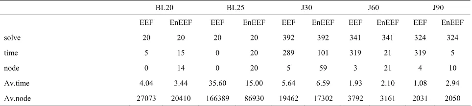
Table 1 reports the results for all instances from the test

sets BL, J30, J60 and J90 that were solved by at least one propagator using dynamic branching. There were 40, 392, 341 and 324 for BL, J30, J60 and J90 respectively. In this table, the line “solve” reports the number of in- stances in which each algorithm found the optimal solu- tion, did so in the fastest time “time”, and generated the smallest search tree “nodes”, using dynamic branching. Line “Av.time” reports the average CPU time (in second) used to reach the optimal solution while line “Av.node” denotes the average number of nodes reported on in- stances solved by both propagators. Both propagators solve the same number of instances in each test sets. As can be observed form Figure 2, using dynamic branching

EnEEF performs the strongest among the two algorithms on instances less than 30 tasks. Unfortunately, the use of a dynamic branching scheme appears to hide the domina- tion of EnEEF on EEF. On instances with more than 30 tasks, EnEEF requires more time for small reduction of tree search.

Here, on BL set (reputed to be highly cumulative [10]), 87.5% of instances were solved by EnEEF with better running time and 85% of instances were solved with smallest search tree. On J30, J60 and J90 instances (re- puted to be highly disjunctive [10]), the performance of the EnEEF is reduced. This result confirms that of Bap- tiste et al. [1] concerning the usage of the energetic rea-

soning on tightness instances.

Table 1. Number of instances in which each algorithm found the optimal solution (solve), did so in the fastest time (time), and generated the smallest search tree (nodes), using dynamic branching. Average runtime (Av.time) and nodes (Av.node) count on instances where both solvers can found the optimal solution are considered.

BL20 BL25 J30 J60 J90

EEF EnEEF EEF EnEEF EEF EnEEF EEF EnEEF EEF EnEEF

solve 20 20 20 20 392 392 341 341 324 324

time 5 15 0 20 289 101 319 21 319 5

node 0 14 0 20 5 59 3 21 4 10

Av.time 4.04 3.44 35.60 15.00 5.64 6.59 1.93 2.10 1.08 2.94

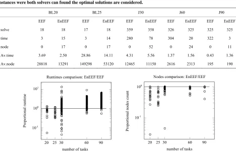
4.2. Static Branching

In Table 2, lines “solve”, “time”, “node”, “Av.time” and

“Av.node” have the same meaning as in Table 1. For

static branching scheme, an instance of BL25 was solved only by the propagator EnEEF in the time available. Two other instances for J30 and J60 respectively was soled by EEF only in the time available. The tests show that the

EEF propagator is faster in a large majority of test in- stances but the EnEEF remains the best on BL test set. As in Table 1, the average running time of EEF is more

than two times the one of EnEEF on the BL25 test set. The same remark can be observed on the average of nodes count of the different propagators on BL25 for both static and dynamic branching scheme. Figure 3

compares (left) the proportional runtime of EnEEF over

Runtimes comparison: EnEEF/EEF

101

100

10-1

20 25 30 60 90

number of tasks

Pr

op

or

tio

na

l r

un

tim

e

102

Nodes comparison: EnEEF/EEF

101

10-1

20 25 30 60 90

number of tasks

Pr

opor

tional nodes

coun

t

10-2

[image:10.595.104.489.191.346.2]

100

Figure 2. Comparison of (left) proportional runtimes of EnEEF over EEF and (right) proportional nodes count when using dynamic branching, sorted by number of tasks of instances.

Table 2. Number of instances in which each algorithm found the optimal solution (solve), did so in the fastest time (time), and generated the smallest search tree (nodes), using static branching. Average runtime (Av.time) and nodes (Av.node) count on instances were both solvers can found the optimal solutions are considered.

BL20 BL25 J30 J60 J90

EEF EnEEF EEF EnEEF EEF EnEEF EEF EnEEF EEF EnEEF

solve 18 18 17 18 359 358 326 325 325 325

time 3 15 3 14 280 78 304 20 322 3

node 0 17 0 17 0 52 0 24 0 11

Av.time 3.69 2.50 28.86 14.11 4.31 5.56 1.37 1.56 0.43 1.36

Av.node 28818 13291 149298 53120 12465 11150 2616 2313 195 190

Runtimes comparison: EnEEF/EEF

101

100

10-1

20 25 30 60 90

number of tasks

Pr

op

or

ti

on

al r

un

tim

e

Nodes comparison: EnEEF/EEF

100

10-1

20 25 30 60 90 number of tasks

Pr

opor

tional nodes

count

Figure 3. Comparison of (left) proportional runtimes of EnEEF over EEF and (right) proportional nodes count when using static branching, sorted by number of tasks of instances.

[image:10.595.61.529.405.705.2] [image:10.595.54.540.428.645.2]

EEF and (right) the proportional nodes count when using static branching, sorted by number of tasks of instances. It appears that the propagator EnEEF subsumes the EEF in almost all test instances. On tests set J30, J60 and J90, EnEEF need more time for a weak reduction of the tree search on instances solved by the propagators.

5. Conclusion

In this paper, it is presented a new filtering algorithm for cumulative resource, hybridization of the extended edge- finding rule and the energetic reasoning. The new algo- rithm is stronger than the extended edge-finding algo- rithm, but weaker than the energetic reasoning and runs in _

 

_n3 _where

n is the number of tasks sharing the

resource. In practice, it is a good trade-off between the filtering power and the running time. Experimental re- sults demonstrate that on a standard benchmark suite, our new algorithm reduces substantially more number of nodes—thus the tree search—than the extended edge- finding algorithm on instances where the number of tasks is less than 30. The time complexity of this algorithm remains too high. Our future work will focus on the re- duction of the complexity of this algorithm from _

 

_n3

to _



_n2_logn



_{using a -tree data structures.}

6. Acknowledgements

The authors would like to thank Pierre Ouellet and Claude-Guy Quimper for providing their paper. We also thank anonymous referees sincerely for their constructive and insightful feedback.

REFERENCES

[1] P. Baptiste, C. Le Pape and W. P. M. Nuijten, “Con- straint-Based Scheduling: Applying Constraint Program- ming to Scheduling Problems,” Springer, Berlin, 2001.

[2] A. Aggoun and N. Beldiceanu, “Extending CHIP in Order to Solve Complex Scheduling and Placement Problems,” Mathematical and Computer Modelling, Vol. 17, No. 7, 1993, pp. 57-73.

[3] P. Baptiste, “Resource Constraints for Preemptive and Non-Preemptive Scheduling,” Master 2 in Computer Science and Operation Research, University of Paris VI, Institut Blaise Pascal, 1995.

[4] L. Mercier and P. Van Hentenryck, “Edge Finding for Cumulative Scheduling,” INFORMS Journal on Comput- ing, Vol. 20, No. 1, 2008, pp. 143-153.

[5] S. F. Betmbe, “Energetic Edge Finder: Propagator of cUmulative Resource Constraints,” Master 2 in Computer Science, University of Yaounde 1, 2012.

[6] R. Kameugne and L. P. Fotso, “Energetic Edge-Finder for Cumulative Resource Constraint,” Proceeding of CPDP

2009 Doctoral Program, Lisbone, 2009, pp. 54-63. [7] R. Kameugne, L. P. Fotso, J. Scott and Y. Ngo-Kateu, “A

Quadratic Edge-Finding Filtering Algorithm for Cumula- tive Resource Constraints,” In: J. H. M. Lee, Ed., CP 2011—Principles and Practice of Constraint Program- ming, Springer, Berlin, 2011, pp. 478-492.

[8] R. Kameugne, L. P. Fotso, J. Scott and Y. Ngo-Kateu, “A Quadratic Edge-Finding Filtering Algorithm for Cumula- tive Resource Constraints,” Extended Version of the CP 2011 Paper, Constraints, Forthcoming, 2013.

[9] “PSPLib—Project Scheduling Problem Library,” Online, 2012. http://129.187.106.231/psplib/

[10] P. Baptiste and C. Le Pape, “Constraint Propagation and Decomposition Techniques for Highly Disjunctive and Highly Cumulative Project Scheduling Problems,” Con- straints, Vol. 5, No. 1, 2000, pp. 119-139.

[11] R. Kameugne, L. P. Fotso and J. Scott, “A Quadratic Extended Edge-Finding Filtering Algorithm for Cumula- tive Resource Constraints,” International Journal of Plan- ning and Scheduling, Forthcoming, 2013.

[12] P. Vilm, “Timetable Edge Finding Filtering Algorithm for Discrete Cumulative Resources,” In: T. Achterberg and J. C. Beck, Eds., CPAIOR 2011—Integration of AI and OR Techniques in Constraint Programming, Springer, Berlin, 2011, pp. 230-245.

[13] P. Ouellet and C.-G. Quimper, “Time-Table Extended- Edge-Finding for the Cumulative Constraint,” Proceeding of the 19th International Conference on Principles and Practice of Constraint Programming, LNCS, 2013, Springer, Berlin, Vol. 8124, pp. 562-577.

[14] R. Kameugne and L. P. Fotso, “A Cumulative Not-First/ Not-Last Filtering Algorithm in O(n2_logn),”

Indian Journal of Pure and Applied Mathematics, Vol. 44, No. 1, 2013, pp. 95-115.

[15] A. Schutt and A. Wolf, “A New O(n2_{logn) Not-First/}

Not-Last Pruning Algorithm for Cumulative Resource Constraints,” In: D. Cohen, Ed., CP 2010—Principles and Practice of Constraint Programming, Springer, Ber- lin, 2010, pp. 445-459.

[16] T. Berthold, S. Heinz and J. Schulz, “An Approximative Criterion for the Potential of Energetic Reasoning,” In: A. Marchetti-Spaccamela and M. Segal, Eds., Theory and Practice of Algorithms in (Computer) Systems, Springer, Berlin, 2011, pp. 229-239.

[17] S. Heinz and J. Schulz, “Explanations for the Cumulative Constraint: An Experimental Study,” In: P. M. Pardalos and S. Rebennack, Eds., Experimental Algorithms, Springer, Berlin, 2011, pp. 400-409.

and OR Techniques in Constraint Programming, 2013, pp. 234-250.

[19] P. Vilm, “Max Energy Filtering Algorithm for Discrete Cumulative Resources,” In: W. J. van Hoeve and J. N. Hooker, Eds., CPAIOR 2009—Integration of AI and OR Techniques in Constraint Programming, Springer, Berlin, 2009, pp. 294-308.

[20] A. Wolf and G. Schrader, “O(nlogn) Overload Checking for the Cumulative Constraint and Its Application,” In: M. Umeda, A. Wolf, O. Bartenstein, U. Geske, D. Seipel and O. Takata, Eds., INAP 2005—Applications of Declarative Programming for Knowledge Management, Springer,

Berlin, 2006, pp. 88-101.

[21] P. Vilm, “Edge Finding Filtering Algorithm for Discrete Cumulative Resources in O(knlogn),” In: I. P. Gent, Ed., CP 2009—Principles and Practice of Constraint Pro- gramming, Springer, Berlin, 2009, pp. 802-816.

[22] Y. Caseau and F. Laburthe, “Improved CLP Scheduling with Task Intervals,” In: P. Van Hentenryck, Ed., ICLP 1994—Logic Programming, MIT Press, Cambridge, 1994, pp. 369-383.