Structural study of heterogeneous biological samples by Cryoelectron Microscopy and image processing

White, Hayley and Ignatiou, Athenasios and Clare, Daniel and Orlova, Elena

(2017) Structural study of heterogeneous biological samples by Cryoelectron

Microscopy and image processing.

BioMed Research International , p.

1032432. ISSN 2314-6133.

Downloaded from:

Usage Guidelines:

Please refer to usage guidelines at

or alternatively

Review Article

Structural Study of Heterogeneous Biological Samples by

Cryoelectron Microscopy and Image Processing

H. E. White, A. Ignatiou, D. K. Clare, and E. V. Orlova

Institute of Structural and Molecular Biology, University College London and Birkbeck, Malet Street, London WC1E 7HX, UK

Correspondence should be addressed to E. V. Orlova; [email protected]

Received 15 September 2016; Accepted 23 November 2016; Published 15 January 2017

Academic Editor: Javier Vargas

Copyright © 2017 H. E. White et al. This is an open access article distributed under the Creative Commons Attribution License, which permits unrestricted use, distribution, and reproduction in any medium, provided the original work is properly cited.

In living organisms, biological macromolecules are intrinsically flexible and naturally exist in multiple conformations. Modern electron microscopy, especially at liquid nitrogen temperatures (cryo-EM), is able to visualise biocomplexes in nearly native conditions and in multiple conformational states. The advances made during the last decade in electronic technology and software development have led to the revelation of structural variations in complexes and also improved the resolution of EM structures. Nowadays, structural studies based on single particle analysis (SPA) suggests several approaches for the separation of different conformational states and therefore disclosure of the mechanisms for functioning of complexes. The task of resolving different states requires the examination of large datasets, sophisticated programs, and significant computing power. Some methods are based on analysis of two-dimensional images, while others are based on three-dimensional studies. In this review, we describe the basic principles implemented in the various techniques that are currently used in the analysis of structural conformations and provide some examples of successful applications of these methods in structural studies of biologically significant complexes.

1. Introduction

Biological molecular assemblies are dynamic machines that can adopt different conformations (local positions) of their domains or subunits in order to perform their functions in the cell. Even when these molecules are purified in vitro, they can be flexible and adopt various possible spatial arrangements of domains in a biocomplex. The multitude of different states is typically identified as sample heterogene-ity. Moreover heterogeneity can also arise in vitro due to differences in buffer, temperature, variable ligand binding, and interactions between molecules or different types of oligomers. For example, a virus sample may contain virions in different stages of maturation [1]; ribosome samples may have subunits in different orientations since they have to move to synthesise polypeptide chains according to the messenger RNA, and a nascent polypeptide chain may have a variety of “prefolding” states within the exit tunnel of ribosomes [2–4]; chaperones are another example of active machines engaged in the dynamic process of refolding substrate molecules and can adopt different conformations during their reaction cycle [5, 6].

X-ray crystallography is a classical technique for deter-mining atomic structures of proteins and protein complexes and relies on the high homogeneity and stability of the sample being crystallised. Often, to facilitate crystallisation proteins may need to be modified in such a way that their flexible regions are removed or substrates are added to stabilize the molecules [7–9]. Consequently, what is seen in a crystal structure may not always be a truthful representation of what is happening in vivo and does not necessarily reflect the biologically active native form. Structural studies using cryoelectron microscopy (cryo-EM) offer methods for examination of molecules/protein complexes in near-native conditions as no crystal needs to be formed [10–13]. In cryo-EM sample molecules are trapped in frozen vitrified solution in nearly native environment at liquid nitrogen temperatures. This technique has improved rapidly over the last few years

and is now able to achieve 2.5–4 ˚A resolution, allowing amino

acids of the polypeptide chains to be seen [14–17].

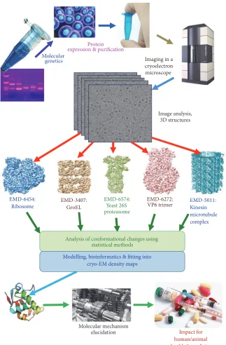
Structural studies using EM are based on imaging of the protein complex followed by a sophisticated computational process (Figure 1). It starts with the automated data collection on the microscope, correction for the distortions present Volume 2017, Article ID 1032432, 23 pages

Molecular genetics

Protein expression & purification

Imaging in a

Image analysis, 3D structures

EMD-6574: Yeast 26S proteasome EMD-3407:

GroEL EMD-6454:

Ribosome

EMD-6272:

VP6 trimer EMD-5011:_Kinesin

microtubule complex

Molecular mechanism

elucidation Impact for human/animal health & medicine

Analysis of conformational changes using statistical methods

Modelling, bioinformatics & fitting into cryo-EM density maps

cryoelectron microscope

Figure 1: Overall diagram of the work flow of structural analysis by cryo-EM.

in the recorded images often induced by the microscope and recording systems, separation of characteristic views of the imaged proteins, and eventually reconstruction of a three-dimensional distribution of electron densities of the protein complex [20]. The electron density maps are then interpreted using methods that dock and refine atomic or homology models or by building de novo atomic mod-els [21–23]. However, if there is significant heterogeneity present in the sample, the electron density may not be well defined in certain areas of the map or may affect the entire density distribution. This will not allow an unambiguous

of this is the ribosome where antibiotics such as kirromycin, sordarin, and others were used to stall the process of protein translation [24–28]. Mutagenesis of the protein has also has been used to produce more stable complexes by removing the flexible regions, which is a standard approach in X-ray crystallography to form good crystals. However, it is not always possible to biochemically trap the most biologically interesting conformations. Several computational techniques in electron microscopy were developed to overcome the problem of sample heterogeneity. All of them are based on statistical approaches that analyse large datasets of par-ticle images. A combination of biochemical methods that will allow complexes to be trapped in a limited range of conformations, together with statistical methods of image analysis, could allow us to link conformations observed in the structures to the movements and specific features in the function of the biological complex [29–31].

Another problem intrinsically linked to the EM imaging of biological molecules is that images in EM are formed by electrons and are registered nowadays with the help of digital cameras. Since biological samples should be preserved in the vacuum system of the microscope they have to be fixed with negative stain or frozen in a thin layer of vitrified ice [20]. These conditions and systems of recording lead to a high level of noise in the images. Another reason for image degradation is beam induced movement. The use of direct electron detectors has helped increase the quantity and improve the quality of the images that we can collect and use. EM images are now recorded as multiple frames by the new direct detectors and these frames can be aligned eliminating the effect of initial strong movement of samples and effects of drift. The averaged image after alignment of subframes removes the noise associated with beam induced movement and low dose [54]. Movie mode processing in combination with the improved performance of the new detectors over all spatial frequencies in the image have now become a standard procedure to obtain higher resolution structures [14, 55–58]. Improvements in technology and image quality have dramatically expanded the capacity of structural analysis by cryo-EM thus not only enabling visualisation of different conformations but also revealing ligands on an atomic level [59, 60]. However, these results did not come at the same time. Development of methods to analyse heterogeneity has taken several decades. The first two methods developed were multivariate statistical analysis (MSA) [61] and principle component analysis (PCA), [62, 63], both of which were initially mostly used to distinguish different views of the same complexes. Later the maximum likelihood (ML) method has been implemented in electron microscopy [45, 46, 64, 65]. Originally these techniques were used to analyse two-dimensional (2D) images but later they have been used in the analysis of three-dimensional (3D) EM maps. During the last decade the bootstrap method and covariance analysis were also used to analyse sample heterogeneity [66, 67]. A number of other papers on statistical methods have been published recently [28, 51, 68–71]. New developments are based on increasingly improved speed of calculations and new multiprocessor technology. Here we aim to provide a review of different statistical methods used in the analysis

of both 2D projection images and 3D maps. However, it should be noted that new approaches are still evolving, new algorithms being proposed, and currently the reader will be provided with a snapshot of the latest developments.

2. Theoretical Background

2.1. Basic Concepts Used in Statistical Analysis. Unfortunately images of biocomplexes recorded in EM are obscured by noise for different reasons. Noise in images is caused by irregularities in the distribution of the negative stain grain used during sample preparation, buffer distribution, vari-ations in ice thickness in cryopreparvari-ations, and low dose conditions where one reduces the electron dose to avoid radiation damage of the sample but this leads to a small number of electrons forming the image. Also beam induced movement/drift of biomolecules is a reason that images became blurry [72, 73]. If the sample has been applied on a carbon film it adds significantly to the level of noise and reduces the intensity of information related to the biological molecule. This has more of a negative effect on the imaging

of small complexes with a molecular weight of less than∼

350 KDa. Another reason for variation in images, which is the most interesting part in these studies, is the existence of the biocomplexes in different phases of their functional action. Now in the era of direct electron detectors, which have significantly improved the recording quality of images compared to the old CCD detectors [55], the problem of differentiating a real signal from noise is still important due to specific features of their sensors [74, 75]. In order to obtain a characteristic view of the molecule, one has to find similar images and then average them to increase the signal-to-noise ratio. With thousands of different particle images it is a challenge to deduce the best criteria according to which particles should be grouped together. A researcher has to firstly remove the effects of noise and distortions in the images and then identify differences in the images due to conformational variations.

2.2. How the Signal Is Related to the Images. The sources of noise mentioned above are not dependent on the features of

the biocomplexes in the study and therefore the noise𝑁( ⃗𝑟)

(noninformative signal) is considered as random, uncorre-lated to the signal (meaningful information), and additive.

So an image𝐼( ⃗𝑟)represents a projection𝑆( ⃗𝑟)of a bioparticle,

where ⃗𝑟is a vector indicating a point in the image and𝑁( ⃗𝑟)

is additive noise at the same point:

𝐼 ( ⃗𝑟) = 𝑆 ( ⃗𝑟) + 𝑁 ( ⃗𝑟) . (1)

as the ratio of themean valueof the signal and thestandard deviation𝜎_noiseof the noise𝑁( ⃗𝑟).

SNR= 𝑆avr

𝜎_noise. (2)

We assume that noise has an average value equal to zero. To fulfil our task for determination of biocomplex structures from images of single particles we need to improve the signal and reduce the noise in order to make the SNR bigger. Averaging of similar images improves the SNR. If we have the

same complex imaged𝐿times (we assume that the particle is

in the same orientation) the signal component is the same at

each measurement. It means that images𝑆_𝑖( ⃗𝑟)are the same

and equal to𝑆( ⃗𝑟):

𝑆_avr= 1 𝐿

𝐿

∑

𝑖=1

𝑆_𝑖( ⃗𝑟) = 𝑆 ( ⃗𝑟) , where𝑖 = 1, 2, . . . , 𝐿. (3)

During registration of images we make another assumption

that noise components𝑁_𝑖( ⃗𝑟)are not correlated to each other

or to the signal and have the same standard deviation𝜎_noisein

all registered images. The result of averaging of𝐿images can

be defined as follows:

𝐼_avr=_𝐿1∑𝐿

𝑖=1

𝐼_𝑖( ⃗𝑟) = 1_𝐿∑𝐿

𝑖=1

𝑆_𝑖( ⃗𝑟) +1_𝐿∑𝐿

𝑖=1

𝑁_𝑖( ⃗𝑟)

= 𝑆 ( ⃗𝑟) + 𝑁avr.

(4)

Since noise is random, therefore𝜎_{noise avr}after summation of

𝐿images is defined as

𝜎_{noise avr}= √1

𝐿

𝐿

∑

𝑖=1

(𝑁_𝑖( ⃗𝑟))2= 1

√𝐿𝜎noise. (5)

Then the SNR will be

SNR_avr= √𝐿 ∗SNR. (6)

The result of summation of𝐿images leads to the

improve-ment of the SNR √𝐿 times, where 𝐿 is the number of

images. However, before averaging, images have to be aligned and evaluated for similarity, since nonaligned and different images will result in the loss of information.

2.3. Concept of the Correlation Function. A low signal-to-noise ratio in EM images of vitreous specimens makes it difficult to see differences in the size and orientation of single images of the particles. However, determination of the particle orientations in images is crucial for 3D analysis. To answer the question “does a set of images represent a biocomplex in the same or different orientations?” one needs to assess their likeness. A general method to assess the

similarity of two objects𝐹( ⃗𝑟) and 𝐺( ⃗𝑟) (images) is to use

a cross-correlation coefficient (CCF), which is defined as a measure of similarity of two functions. The functions can be

multidimensional, where the variable ⃗𝑟is a multidimensional

vector and 󸀠⃗𝑟 is a shift of the function𝐺( ⃗𝑟)with respect to

the function𝐹( ⃗𝑟). To assess the level of similarity, one has

to multiply the two functions point by point, and the results of each multiplication are then summed; this operation is performed for different shifts. The location of the maximum of this new CCF function which depends on the shifts will

give information on how one image𝐺( ⃗𝑟)is displaced with

respect to the image 𝐹( ⃗𝑟) and the height of the output

correlation peak indicates the degree of their similarity. The CCF should be normalized using the product obtained from the multiplication of each function by itself.

CCF( ⃗𝑟󸀠) = ∫ 𝐹 ( ⃗𝑟) 𝐺 ( ⃗𝑟

󸀠_{+ ⃗𝑟) 𝑑 ⃗𝑟}

√∫ 𝐹 ( ⃗𝑟) 𝐹 ( ⃗𝑟) 𝑑 ⃗𝑟∫ 𝐺 ( ⃗𝑟) 𝐺 ( ⃗𝑟) 𝑑 ⃗𝑟. (7)

The height of the CCF maximum serves as a measure of the image similarity and is named as the cross-correlation coefficient (CCC). If images are identical then the CCC is

equal to 1. The value of ⃗𝑟󸀠 where the CCF has the

maxi-mum indicates the coordinates of the best correspondence between the two images. Images can then be sorted using the CCF between all possible pairs to assess similarities and differences, a task that is not difficult until one has tens of thousands of images and at that stage it becomes computationally expensive.

3. Multivariate Statistical Analysis

3.1. Principles of MSA. Work in the EM field using multivari-ate statistical analysis (MSA) was initimultivari-ated by van Heel and Frank in 1981/1982, who combined their efforts to solve the problem of recognising/distinguishing characteristic (reli-able) views in negatively stained samples with MSA. It was used to find variations due to differences in structure rather than those due to different orientations [77–79].

The main advantage of multivariate statistical analysis (MSA) is its ability to examine relationships among multiple variables at the same time. Different versions of this analysis have been implemented, but all are based on reducing the number of variables in such a way that only the most significant ones are used. The question is how to find the essential variables (parameters) and to avoid the influence of unimportant parameters such as noise. One of the most helpful descriptions of MSA has been given by van Heel and coauthors [80].

Images x y

#1

#2

#3

#4

#5

100 20

80

80 20

40

80 60

60

#6

#7

#8

#9

#10

0 100

20

20 40

100

40 60

40 80

x y

2 1

3 5 4 8

6

10

9

7

100

0 20 40 60 80

0 100

20 40 60 80

100

(a)

Value 1

V

al

ue 2

Class 1 Class 2

10 8

1 2 3 4 5 6 9

Class 1 Class 2

7

(b)

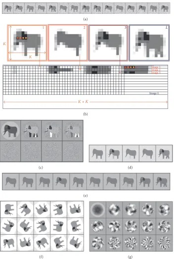
Figure 2:Multivariate Statistical Analysis.(a) Left: ten images, each consisting of 2 pixels. Right: each image is represented as a vector in 2-dimensional space according to their grey values. (b)Hierarchical Classification.The left panel shows the sequential combination of vectors according to their closeness. The initial classification of images starts by forming small classes which include images that are close to one another in multidimensional space and then the size of the group is progressively increased by merging with dimensional other surrounding smaller groups that are in close proximity to each other (see the text). Images that are too far from each other form new separate classes. In the example shown in panel (b) the process of forming two classes is represented by the blue and green ovals which have varying degrees of colour intensity. The light and dark coloured ovals correspond to the initial and final steps of classification, respectively. The right panel shows a tree of HAC. The starting point is 10 classes which correspond to the number of single images in the dataset. The cut-off point is shown by the dashed red line if 2 classes are required and this corresponds to the two classes shown in the left panel.

of which form a data cloud (see [80]). The images or volumes that are similar to each other will form a cluster (a class) of vectors with their ends in close proximity to each other; these small differences are typically induced by noise (Figure 2(b), left). However, if the distances between the vector ends are large (compared with the length of the vectors) or they make another cluster of points, sufficiently remote from the first one, they could represent a group of images (or volumes) that have different features related to conformational changes or from a different angular projection (Figure 2(a), right). The essence of the MSA approach is in the assessment of variations within the cloud of points and the determination of variations which are significant or not. These variations can be ranked according to the distances found between points

representing the dataset. Categorized variations are used as a new system of coordinates for the entire dataset and using only the most significant one of them leading to the reduction of variables taken into consideration during analysis. This allows us to concentrate on the most important variations found in the dataset and to ignore sources of insignificant variability (typically related to noise in images).

How can one do such an estimation of variations for large datasets? Mathematically the entire dataset can be

represented as a matrixD where each line corresponds to

one image and its length is defined by the size of the image (or a volume; see Figures 3(a) and 3(b)). The number of lines corresponds to the number of images. However, the number

(a)

3 2

1

K

Image 2 Image 3

Image L

Image 1

L

K

K ∗ K

(b)

(c) (d)

(e)

(f) (g)

image𝐾 ∗ 𝐾which makes the matrixDnot square. Having so many variables the problem of comparison of images can be solved by determination of eigenvectors of the covariance

matrixCwhich is defined as [81]

C=D𝑇∗D− ⃗𝑂𝑇∗ ⃗𝑂, (8)

where ⃗𝑂is a vector representing the average of all images

in the dataset,D𝑇is transpose of the matrixD, and ⃗𝑂𝑇is a

transpose of the vector ⃗𝑂:

C ⃗𝑉_𝑗= 𝛾_{𝑗 𝑗}⃗𝑉. (9)

If the vectors ⃗𝑉_𝑗multiplied on matrixDscale the matrix

by coefficients𝛾_𝑗 (scalar multipliers) then these vectors are

termed as eigenvectors, and scalar multipliers are named as eigenvalues of these characteristic vectors.

The eigenvectors reflect the most characteristic variations in the image population [78, 80, 82]. Details on eigenvector calculations can be found in van Heel et al., 2016 [80]. The eigenvectors (intensity of variations in the dataset) are ranked according to the magnitude of their corresponding eigenvalues in descending order. Each variance will have a weight according to its eigenvalue. Representation of the data in this new system coordinates allows a substantial reduction in the amount of calculations and the ability to perform comparisons according to a selected number of variables that are linked to specific properties of the images (molecules).

MSA allows each point of the data cloud to be represented

as a linear combination of eigenvectors _𝑖⃗𝑉with certain

coef-ficients𝐴_𝑖. The number of eigenvectors𝐽used to represent

a statistical element (the point or the image) is substantially smaller than the number of initial variables in the image.

𝐼 ( ⃗𝑟) = 𝐴1󳨀→𝑉1+ 𝐴2󳨀→𝑉2+ ⋅ ⋅ ⋅ + 𝐴𝐽󳨀→𝑉𝐽, (10)

where𝐽 ≪ 𝐾 ∗ 𝐾and𝐾is the image size.

Clustering or classification of data can be done after MSA in several ways. The Hierarchical Ascendant Classification (HAC) is based on distances between the points of the dataset: the distances between points (in our case images) should be assessed and the points with the shortest distance between them form a cluster (or class), and then the vectors (their end points) further away but close to each other form another cluster. Each image (the point) is taken initially as a single class and the classes are merged in pairs until an optimal min-imal distance between members of a single class is achieved, which represents the final separation into the classes. The global aim of hierarchical clustering is to minimize the intraclass variance and to maximize the interclass variance (between cluster centres) (Figure 2(b), right). A classification tree contains the details of how the classes were merged. There are a number of algorithms that are used for clustering of images. Since it is difficult to provide a detailed description of all algorithms in this short review, the reader is directed to some references for a more thorough discussion [63, 80, 83– 85]. In Figure 2(b), 10 classes (corresponding to a dataset of 10 single images) have been chosen at the bottom of the tree and these have been merged pairwise until a single class is

reached at the top of the tree (Figure 2(b)). The user can then decide on the number of classes and thus where the tree will be cut.

Another idea of separation of images into classes is based on the opposite concept, where initially all data points are considered as one class and the distances of each data point from the centre of the cluster are assessed and the class is separated into two where the points are closer to each other (divisive hierarchical clustering). It should be noted in EM that agglomerative algorithms are mostly used. Both procedures are iterative which is continued until there is no movement between the class elements.

In 2D clustering analysis (CL2D) Sorzano and coauthors suggested the use of correntropy as a similarity measure between images instead of the standard least-squares distance or, its equivalent, cross-correlation [86]. The correntropy represents a generalized correlation measure that includes information on both the distribution and the time structure of a stochastic process (for details see [87]).

3.2. Illustrations Using Model Data. Typically a dataset col-lected by EM has thousands of images and it is important to assess which differences are significant and to sort the images into the different populations based on these significant differences. A simple example of the classification of a set of two-dimensional (2D) images using HAC is shown in Figure 2. In this example we have a population of 12 elephants that have variable features (Figure 3(a)). For the MSA the following procedure is performed: each image of an elephant

consists of𝐾columns and𝐾rows (Figure 3(b)). We represent

each elephant from our raw dataset (Figure 3(b)) as a line

of the matrix D, where the first row of pixels in elephant

1 represents the start of the first line in the matrix D, and

then the density values of the second row follow the first row along the same line in the matrix. This process is repeated until all rows of elephant 1 have been laid out in the first row of the matrix (Figure 3(b)). The pixels of elephant 2 are placed in the matrix in the same way as elephant 1 but

on the second line of matrix D. This process is repeated

are darker as they correspond to the highest variation in the position of this leg in the images of the elephants. The remaining four eigenimages have the same appearance of a grey field with small variations reflecting interpolation errors in representing fine features in the pixelated form.

At the first try of the classification (or clustering) of elephants we have produced 5 classes that were based on first four main eigenimages. Here we see four different types of elephant (classes 1, 2, 3, and 5) (Figure 3(d)). However, if we choose 10 classes, we have five distinct populations (classes 1, 2, 4, 9, and 10) (Figure 3(e)). Some classes can be repetitive; for example, 1 and 7 are nearly the same. Such small differences could be due to noise and the weight of these small vectors can have a minor role.

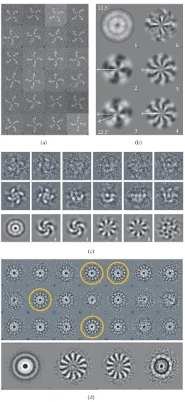
3.3. Usage of MSA for Determination of Symmetry. When doing structural analysis one has to check what sort of symmetry can be expected in the complex. MSA is commonly used to determine the rotational symmetry of complexes. Typically the rotational symmetry of a complex is only seen in its end views so these views must be separated from the side views and oblique views for this analysis to work. Even if the number of end views is not very high one can artificially increase their numbers by applying random in-plane rotations to generate more end views (Figure 3(f)). It is important to mention that the images have to be centred for symmetry analysis; otherwise the eigenimages will reflect variations due to displacements of images. In Figure 3(g) the eigenimages of the unaligned elephants shown in Figure 3(f) display some sort of featureless images with a hint of symmetry which is related to rotations of images within the frames. Eigenimages 2 and 3 look rather similar

but are rotated by 90∘, indicating that they are orthogonal

vectors and do not provide symmetry information. However, if we look at a well centred model with 4-fold symmetry (Figure 4(a)) eigenimages demonstrate clear 4-fold symmetry

(Figure 4(b)). When real data is used, for example, 𝛼

-latrotoxin, the 4-fold symmetry is seen in the class averages and the eigenimages, calculated only for the end views (Figure 4(c), [88]). This technique also works for higher rotational symmetries as demonstrated by the connector complex from bacteriophage SPP1 (Figure 3(d), [89]). In this complex 12-fold symmetry is clearly visible in both the class averages and the eigenimages.

It is important to mention other approaches used for the determination of rotational symmetry. Crowther and Amos [90] introduced rotational power spectrum analysis of indi-vidual particles. This technique has been successfully used in many studies. However, this estimation of the symmetry is typically affected by low SNR in single images and especially for images taken in cryoconditions. Marco and coauthors described an example of the rotational symmetry assessment which uses rotational power spectra of many different end

views of single particles. This is followed by a 𝐾 nearest

neighbour classification, statistical analysis with eigenvectors, and a circular harmonic analysis ([91] and references therein). These approaches are implemented in SPIDER, XMIPP, and EMAN2 [34, 41, 43].

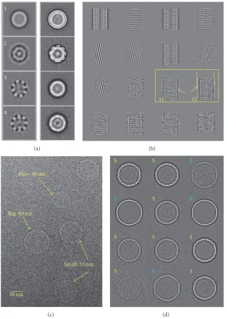
3.4. Statistical Analysis of Particles of Different Sizes. MSA is also a powerful technique for visualising size differences in a population of images. To reveal variations within a dataset related to orientation or conformational changes, the 2D images should be well aligned. The quality of the alignment can be assessed by visual examination of the eigenvectors obtained during statistical analysis. In the case of possible variations in sizes the dataset should be centred. Visual inspection of eigenvectors can indicate if the particles differ in size; in this case one can see eigenvectors with a characteristic pattern of concentric rings. The variations in overall size can be evaluated by calculation of the differences between classes and the first eigenimage (which is an average of all images). A characteristic feature of size variation in a dataset is a ring that can be seen in the second eigenimage from a dataset of Hsp26 (Figure 5(a), left panel, [33]). Then images comprising the classes with the positive difference in the outer rim (large particles) should be extracted in one subset while the images that constitute the classes with the negative outer rim (small particles) should be extracted into another subset (Figure 5(a), right panel). That will create two more homogeneous subsets. It will be natural that some differences will not show clear positive or negative outer ring that will say that the images corresponding to these classes were not separated and should be selected into the third subset and subjected to a new round of centring and subclassification. It is possible that there can be more than two size groups of molecules. This hypothesis can be verified by MSA again and images can be separated according to the eigenvectors.

Minor variations in the size of the particles are often not visible in micrographs but they limit the resolution if the particles were picked on apparent size alone and combined in the same dataset as heterogeneity would still be present. Statistical analysis has revealed that the spherically shaped molecule has two conformations, both with tetrahedral

symmetry, but differing in size by about 10 ˚A [33]. Care

has to be taken, however, that the characteristic ring is not caused by poor alignment of the molecules. The helical barley stripe mosaic virus (BSMV) also shows size variations in its eigenimages, but, rather than a circle as seen in Figure 5(a), it can be seen by the presence of black peripheral borders in eigenimage 12 (Figure 5(b), [18]).

Another example where MSA and classification has revealed variations in the size of a large complex is the study of the bacteriophage SPP1 procapsids (Figure 5(c)) where three large size differences were visible on the micrograph [19]. Alignment and calculation of eigenimages using MSA revealed minor size variations and helped to verify an improved separation (Figure 5(d)). In this case four of the classes have a size compatible with the “big” procapsid of Figure 5(c) and eight with the “small” procapsid.

(a)

1

2

6

3 4

5

22.5∘

22.5∘

(b)

4 4 8 8

(c)

(d)

1

2

3

4

(a)

11 12

(b)

Pico: 40 nm

Big: 60 nm

Small: 55 nm

30nm

(c)

S

S

B

S

S

S B

S

B B

S S

(d)

Figure 5:Eigenimages-Size Variation.(a) Eigenimages of Hsp26 are shown in the left panel. Eigenimage 1 represents the total sum of the dataset. Eigenimage 2 shows the continuous outer circle which indicates the characteristic size difference range within the dataset. The right panel shows the entire dataset separated into four classes via MSA by only using these first four eigenimages. The big class is highlighted with a white circle around its perimeter, the small class is highlighted with a dashed white circle, and the remaining two classes represent a mixture of large and small Hsp26 images. (b) Eigenimages of BSMV. The size difference is shown in images 11 and 12 (adapted from [18]). (c) A representative micrograph showing the heterogeneity of the SPP1 bacteriophage procapsids where different sizes are clearly seen [19]. (d) The classes of the procapsid images are labelled according to their size, big (B, in blue) and small (S, in yellow).

to 8 3D structures which were calculated from 200 to 400 images. The use of MSA in this classification method allowed differences in the three main domains to be seen. Different orientations were found in the stalk of U4/U6.U5 tri-snRNP, the left head domain of the U5 subunit of tri-snRNP, and the U5 foot domain [30].

3.5. Statistical Analysis of Particles with Variable Ligand Occupancy. If the particles have a different composition and

incomplete occupancy of a substrate, it will be useful to start from multireference alignment so that all images will be brought into orientations defined by the initial model. The images should then be separated into subsets corresponding to the more characteristic views and subjected to MSA. If a substrate has a sufficiently large mass (a component that

is≥20 kDa and not stably bound to the biocomplex) then it

(a)

1

2

3

(b)

Figure 6:Eigenimages-Substrate Binding.(a) GroEL bound to the substrate rhodanese with the raw images (top) and eigenimages (bottom). Eigenimage 5, highlighted with a yellow box indicates heterogeneity in thetrans-ring which is related to the binding of rhodanese (adapted from [5]).(b) Three of the 12 orientation classes (column 1) from GroEL-rhodanese complex after MSA based on the eigenimages, the first six of which are shown in (a). The eigenimages of these classes are shown in columns 2–5 and the heterogeneity in thetrans-ring is highlighted with a yellow box (from [5]).

location in different eigenimages will depend on orientations of the particles in images. The data can be separated into subsets using the eigenvectors (images) that show the varia-tions in question and then 3D reconstrucvaria-tions for each subset can be obtained, followed by assessment of the differences by calculations of difference maps [5].

MSA was used to detect the heterogeneity in the binding of Groel-GroES-ADP with substrate rhodanese [5]. No signs of heterogeneity can be seen in the raw images (Figure 6(a), top panel), but eigenimage 5 (Figure 6(a), bottom panel) indicates, by the two bright spots in the bottom of the image,

that there is variation in density in thetrans-ring reflecting

heterogeneity due to partial occupancy by the substrate. Further still, eigenimages 5 and 6 show signs of orientation variation by black and white perimeter outlines so they are not the best candidates for a separation based solely on these eigenimages. A further classification was carried out based

on the first 11 eigenimages, but excluding eigenimage 5, to remove any bias towards the ligand. After this MSA, 12 classes were produced and the eigenimages obtained from these new classes showed the bright spots indicating density variation in thetrans-ring (Figure 6(b), highlighted in yellow boxes). The data was then further classified into 3 subclasses based on the

eigenimages that showed local variations in thetrans-ring [5].

4. Maximum Likelihood Estimation Method

4.1. Basics of ML. This approach was applied to EM studies for the first time by Sigworth [64]. The Maximum Likelihood Estimation (ML) method is used to find a model that has

the highest probability of representing a dataset𝐼_𝑖( ⃗𝑟), where

𝑖 = 1, 2, . . . , 𝑁, and𝑁is a number of images in the dataset (the approach can be applied to both 2D and 3D data). The ML method is based on the assumption that the dataset

represents many copies of images of𝑀structures (or images

of several structures) to which noise (a general assumption that this is Gaussian noise) has been added. Our goal is to

maximize the probability𝑃, such that the subdataset𝐼_𝑚( ⃗𝑟)

corresponds to the model𝑀_𝑚 with a set of parameters 𝜃.

These parameters are an estimate of the true structure, the noise, and any transformations involved.

Maximizing the likelihood is equivalent to maximizing

its logarithm𝐿. Assuming that individual images𝐼_𝑖( ⃗𝑟)are

independent, this function can be written as a sum of

likelihood logarithms for all images𝐼_𝑖( ⃗𝑟). This maximization

is achieved by optimizing the log-likelihood function,𝐿(𝜃),

given by the equation [64]

𝐿 (𝜃) =∑𝑁

𝑖=1

ln𝑃 (𝐼_𝑖( ⃗𝑟) | 𝑀_𝑚, 𝜃) . (11)

Typically a few random images from the dataset are chosen by the user as a starting point for the analysis,

sometimes referred to as “seeds.” Each particle image 𝐼_𝑖

in the dataset is assigned a probability that it represents a

structure𝑀_𝑚 and particle images with a similar probability

are assigned to the same class of images𝐼_𝑚.

Refinement and reassigning images to classes are based

on the probability𝑃that is linked to the correlation function

and performed using newly assessed parameters𝜃(e.g., new

angles, shifts, and correlation to projections of one of the models) with respect to the new classes obtained. An image may have good correspondence, as shown by the CCC with several projections of one model and possibly with some projections of another model. So there are several possibilities of assigning the image to one model or another. Here the probability of this image belonging to one or another model will be defined by the height of the correlation with the projections and a number of local best projections with good correspondence. The higher the CCC is an indication

that the image has a higher probability𝑃 and that it likely

corresponds to this given model. The classification is usually iterated a number of times resulting in a different quantity of particles per class each time. The number of particles chosen can be increased, so long as new information is obtained in the output class averages. It has been found that 200–300 particles per class provide a good basis for initial reconstructions, though for negative stain data fewer particles per class can be used. If there are too few particles per class, then the alignments and classification become less accurate in ML [94]. During the calculation, all particles are compared to all references in all possible orientations and weighted probabilities obtained for each case. Weighted class averages

are then calculated and used as the input in the next round of optimization.

This is a slower method than a correlation based align-ment but does produce good convergence. The calculation can be speeded up if prealigned particles are used and a binary mask is applied so that only areas where variations occur are included. Such masking provides an additional advantage in that the variable regions will not interfere with the area of interest and more accurate classes could be obtained. In 2007 Scheres and coworkers extended the ML method for both 2D and 3D to overcome two drawbacks: CTF had not been considered and only white noise was used [45, 46].

The ML 3D analysis requires a 3D starting model, the choice of which has a significant impact on the success of the classification. This starting model has to be determined by other methods prior to any ML classification. Often the initial model can be derived using a similar structure, either by creating a low resolution map from PDB coordinates or by using another related EM map. When this is not available, then a map can be calculated using angular reconstitution [95] or Random Conical Tilt (RCT, [96]). If RCT is used, 2D images can be classified and a 3D model calculated for each class but the missing cone of data limits the resolution obtained from this method. The 3Ds from RCT subsets can be aligned in 3D space using an ML approach where the starting reference could be Gaussian noise [97]. In order to avoid model bias, it is helpful to use a model that incorporates all the different structures in the dataset (the average one). Further complications arise if the model is not low-pass filtered. Often small details (or high frequencies) give local minima; however too many low frequencies can give blobs that will not refine. If the starting model has come from a PDB file or from a negative stain EM map, it is recommended to refine the starting model against the complete dataset; this will remove any false features and give better convergence.

A number of models or “seeds” are needed for the ML 3D classification as it is a multireference alignment. If four starting seeds are used, then the whole dataset can be divided initially into four random subsets and each one refined against the starting model created from the PDB, EM, or other method. As in 2D classification, the number of seeds has to be chosen carefully and should correspond approximately to the expected possible conformations of structures, but their number may be limited by the size of the dataset or computing power available. Hierarchical classification can also be used. For example, an initial classification into four classes of a ribosome dataset gave two intact and two broken structures. The particles in the intact classes were then separated into four more classes, which showed two classes with strong RNA density while the other two did not have any tRNA densities corresponding to tRNA. The two classes with strong tRNA density were further classified into four more classes, and these four classes showed alternative tRNA conformations [94].

ML is a computationally expensive procedure and Scheres and coauthors [65] introduced a faster search algorithm by

reducing the search space. Since the assignments of𝐾_𝑙and𝜃

are independent, the probability of assigning image𝐼_𝑖to the

over a range of possible rotations and translations of𝐼_𝑖during the first iteration of the examination; all translations are saved in the data file of processing results. Reduction of the calculation time can be achieved by further iterations, if the

probability of 𝐼_𝑖 to be assigned to𝐽_𝑙 is not significant, and

then it is assumed that none of these translations will increase the probability that the image corresponds to the reference images used in the next iteration. Therefore integration over the translations is not performed. Scheres with coauthors [65] obtained almost identical results using this fast method compared to the full search, but the fast method was 6.5 times faster when compared to the full-search protocol. Nonetheless, in all cases where ML is used, care must be taken in choosing the search space to avoid being trapped in a local minimum. An overview of maximum likelihood has been given by Scheres [94] and Sigworth with coauthors [98].

4.2. Examples of Usage of ML in Analysis of Heterogeneity. This technique has been used for a variety of different complexes in EM. Lee et al., 2011 [99], applied the technique to helical objects: firstly to a homogeneous dataset of TMV which had one class and secondly to a NaK ion channel. The NaK ion channel had two classes, each with a different helical

symmetry, and resolutions of 7.84 ˚A and 7.90 ˚A were obtained.

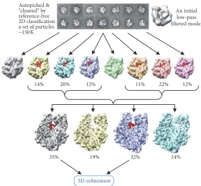
Wang and coauthors [71] were able to resolve conformational changes in viruses using time resolved experiments. The structures have shown different stages of the maturation of Nudaurelia Capensis Omega Virus, an RNA virus. This virus had been previously studied using difference maps [100] but this procedure restricted the difference to a small region of the structure. However, the use of maximum likelihood allowed the authors to view more steps during the maturation process. RELION implements a modified version of ML, where the adaptive expectation maximization algorithm is used thus allowing faster processing [37]. The algorithm has been described by Tagare et al. [101]. RELION is successfully used in the analysis of conformational changes of large biocomplexes. This approach is based on a few major steps. Firstly data cleaning is performed by 2D classification for the removal of bad particles which do not correspond to the fully assembled complexes or badly misaligned images. Images which belong to bad classes are eliminated from further processing. Then the 3D ML classification is applied to the cleaned dataset and typically 2 to 8 structures are produced. These maps are then examined in the designated areas for the presence of any expected ligands and for the case of the ribosome this would be elongation factors or different tRNAs (Figure 7). Images which were used to obtain structures with similar features are extracted into separate subsets and sub-jected to the next round of 3D classification. Subseparation of the dataset allows one to distinguish different states of large biocomplexes and refine their structures to high resolution [15, 102, 103].

ML has also shown to be effective in tomography. Scheres and coauthors [47] first tested their approach on GroEL and GroEl-GroES models. Electron density maps were calculated at 2.5 nm resolution from PDB coordinates of GroEL and GroES. Images of GroEL and GroEl-GroES were randomly selected from all datasets and 200

subtomograms were calculated. Three classes were obtained using a maximum likelihood approach combined with unsu-pervised alignment followed by classification. Two classes showed 7-fold symmetry, one class contained GroEL, and one contained a GroEL-GroES complex, while the third class could not be assigned to either GroEL or GroEL-GroES. Scheres and coauthors [47] then extended their method to a p53 mutant in complex with dsDNA starting with only 40 RCT reconstructions. The two averaged models obtained the following: the structure with C2 symmetry was similar to an independent reconstruction using common lines. A structure without any imposed symmetry differed from the C2 structure by a movement in the top part of the structure.

5.

𝐾

-Means Clustering

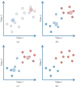
K-means clustering is used to separate the image data into a number of possible structural conformers. Centroid-based K-means clustering is based on the concept that there is a central vector, which may not necessarily be a member of the dataset, around which the subdata can be grouped.

The number of clusters is user defined, for example, to𝐾;

the initial 𝐾 seeds are set typically randomly (Figure 8).

The optimization task is to find such𝐾 centres of clusters,

such that the data objects (images) of a class (cluster) will be located to the nearest cluster centre [63]. If we have a

number of images(𝐼₁, 𝐼₂, . . . , 𝐼_𝑁), where each image is a

d-dimensional real vector (see above in the MSA section), K-means clustering aims to separate the𝑁images into 𝐾

subsets, where𝐾 ≪ 𝑁and𝐼_𝑛 ∈ {𝑆₁, 𝑆₂, . . . , 𝑆_𝐾}. Separation

of images 𝐼_𝑖 into subsets𝑆_𝑘 is based on the minimization

of within-cluster sum of squares (WCSS) (sum of distance

functions of each point in the cluster to𝐾_𝑘centre). Therefore

a set of observations (our data𝐼_𝑖) is divided into a series of

subsets𝑆_𝑘, under the constraint that the variance of the WCSS

should be minimized. In other words, its objective is to find

the minimum arg min_𝑠 of possible distances between a centre

and data elements (images):

arg min

𝑠 =

𝐾

∑

𝑘=1

∑

𝐼∈𝑆𝑘

󵄩󵄩󵄩󵄩𝐼𝑘avr− 𝐼𝑖󵄩󵄩󵄩󵄩2, (12)

where 𝐼_𝑘avr is the mean of images in the class 𝑆_𝑘. The

proximity between images 𝐼_𝑘avr and 𝐼_𝑖 is estimated by the

distance between the end points of the vectors (Euclidean distance).

Autopicked & “cleaned” by reference-free 2D classification a set of particles

22%

20% 12% 11% 12%

14%

32%

35% 19% 14%

3D-refinement

An initial low-pass filtered model

~150K

Figure 7: ML procedure in the analysis of conformational changes of biocomplexes. Raw images are firstly assigned initial orientation angles using the initial model. That is typically done by projection matching. Then the ML approach is used to obtain 6 to 8 reconstructions. Each 3D model is visually examined in the area of interest; for a ligand presence, in this case the bound tRNA is highlighted in red. Images which were used to obtain the models with tRNA are extracted and subjected to the next round of classification. The following step involves extracting images corresponding to one or another conformation and then followed by refinement. The percentages below the structures in the top row indicate fractions of images from the entire dataset used to calculate these models, while in the second row the percentages are taken from the number of images supposedly containing the bound tRNA.

achieved (Figure 8(d)). The Euclidean distance is commonly used to assess a level of similarity (closeness) between images, but it is typically affected by noise in images. Normalization and dimensionality reduction like the coarsening of data are helping to improve the quality of clustering and speed up the calculations.

More recently new approaches where the distance metric learning from training data is used improve the prediction

performance of𝐾-means clustering methods [70]. Recently

Extended Nearest Neighbour (ENN) Method for pattern recognition has been described where the distance-weighted approach is used. Improvement of the efficiency in ENN is achieved by a preprocessing step where a subset (randomly selected) of the dataset is used to make a classification deci-sion. Then all elements in the dataset are ranked according to the distances from the initial classes and assignment to a class is done to maximize the intraclass coherence [104].

6. Three-Dimensional Covariance

MSA and ML methods are widely used for both the global quality assessments of images (or maps) and for the examina-tion of local variaexamina-tions. Such informaexamina-tion on local, real-space, differences between the maps is essential for understanding if the changes are related to different conformations or due to

noise. Assessment of the 3D variance between multiple 3D structures provides an effective tool to assess the stability of each element in the structures. In the covariance matrix used in EM, a single row contains the covariance between voxels of one volume with the corresponding voxels of another volume. If the voxel is located in the area of a ligand that is present in all maps, the matrix will show large covariance of this ligand area with the ligand areas in other maps, but if in other structures ligand is absent then the covariance will be weak and that will indicate that there are changes caused by unstable ligand binding. However, the local differences revealed by the value of voxel-by-voxel real-space variance may arise from errors in the reconstruction procedure such as bad alignments or an uneven distribution of angles defined for the images [68].

Value 1

V

al

ue 2

(a)

Value 1

V

al

ue 2

(b)

Value 1

V

al

ue 2

(c)

Value 1

V

al

ue 2

(d)

Figure 8:K-Means Clustering.(a) Two initial seeds are randomly placed within the data. (b) Step 2 indicates positions of the averages of images that are nearest to the seeds. (c) The averages are then recalculated based on the assignments in step 2. Steps 2 and 3 are reiterated; (d) shows the final classes.

between structures or, in the case where there are no discrete conformations, current reference-free classification schemes may not always be effective. In order to overcome these problems, techniques that examine the information inside the covariance matrix are being developed. A major obstacle in this approach is the large size of the matrix that should be analysed for major variations. To make the process of calculation faster it was suggested that the 3D maps should be coarsened [65].

The calculations of 3D variance of maps help to find the arias with high variations. The covariance of a 3D map indicates how variations in the density at one voxel correlate with variations in another voxel. Conformational changes where a structural element is found in different positions in two structures would come from a negative covariance between these two locations in the map. Calculations of the covariance of maps is computationally highly demanding (the

covariance matrix of a 106-voxel map will have 1012 entries)

but techniques have been developed recently to identify the principal components of the covariance [28, 49, 105]. Anden and his collaborators [39] optimized the algorithm by using a conjugant gradient method. The conjugate gradient method is an iterative algorithm, allowing the best approximation of the solution of large systems of linear equations to be found [106]. This has the advantage of allowing a nonuniform distribution of angles where the CTF can be taken into account.

7. Bootstrapping

St

ep 2

St

ep 1

St

ep 3

St

ep 4

M imag

es p

er 3D

1 2 ··· ··· L

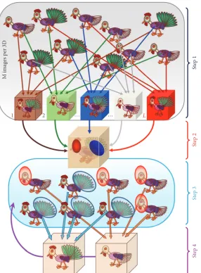
Figure 9:Bootstrapping.A representative set of chickens with different tails and head positions. During step one each of𝐿subsets of M images was picked to make𝐿reconstructions. During step 2 the variance within𝐿reconstructions determines the most significant differences in the head (green) and tail (red) positions. The result of the classification of images shown in step 3 is done by analysing the level of variance in areas defined in step 2 (highlighted by red and blue circles). The two reconstructions generated are then used as the input to carry out the refinement using the focused classification (step 4).

bootstrap estimate. A histogram of these means will indicate how much the mean varies. Areas of variance in the maps can then be visualised. In Figure 9 (step 2) the red and green spheres correspond to the variations in head position and tail type, which are highlighted in the model below. The following step of the procedure involves masking out areas surrounding the region of interest with high variance. These masks are then projected at different angles, determined for the images, producing a set of 2D masks which are then used to eliminate stable features and classify the 2D images according to variations of the selected region. In step 3 all the 2D images are sorted into subsets according to their

Euler angles and a K-means clustering is used for each

subset in the areas of variance determined from the 2D masks. The number of groups obtained for each set usually corresponds to the number of different structures expected. A multireference competitive 2D alignment is performed

against 2D projections of the models obtained in step 4 allowing for structure refinement. Then the corresponding new 3D structures are calculated. The refinement is per-formed iteratively with images corresponding to these new 3D structures until one ends up with structures for each conformation (Figure 9).

correction. The next step included the standard bootstrap procedure of calculating a number of different maps for each dataset followed by calculations of two 3D variance maps. The maps from the CTF corrected 3D produced the variance found originally, but the map from the uncorrected data had strong artefacts making it difficult to find regions of real variance. This computational experiment indicates the importance of the CTF correction for the improvement of a resolution in structures [68].

Liao and Frank [35] proposed an approach for separation of different conformations using the bootstrap technique and

tested it on anE. coli70S ribosome dataset (previously been

subjected to the ML technique, [45, 46]). They used five eigenvolumes and looked for two classes. The difference in the two structures was immediately obvious as EF-G was visible in one map but not on the other and the L1 stalk was in a different position in both maps. Penczek with

coauthors [28] analysed the stalk area of a 70S∗tRNA∗

EF-Tu∗GDP∗kirromycin ribosome complex and found four

separate structures: two represent the main conformation with or without the E-site tRNA while the others show the rotated conformation with a P/E hybrid site tRNA. Simonetti et al., 2008 [93], determined the structure of a 30S

ribosome initiation complex with tRNA and fMet-tRNAfMet

and initiation factors IF1 and GTP-bound IF2. They found five different structures that were statistically relevant ranging from 8% to 40% of the dataset. All structures contained tRNA

and fMet-tRNAfMet and IF1; however, the conformation of

fMet-tRNAfMetwas different in the structures where 1F2 was

absent.

8. Neural Networks

An artificial neural network (NN) is a concept, based upon the NNs in animals, particularly in the brain, and is used to estimate functions with a large number of inputs and classify them into certain groups. A self-organizing map (SOM) algorithm [107] appeared to be efficient in image analysis. The dataset of EM images represent the input for the self-organizing map (network). Here it is assumed that the dataset

of images are represented as vectors𝐼_𝑖( ⃗𝑟) : 𝐼_𝑖 ∈ 𝑅𝑛, where

𝑖is an index of the image within the dataset sequence and

there is a set of variable reference vectors (in our case a set

of images)𝑀_𝑚( ⃗𝑟) : 𝑀_𝑚 ∈ 𝑅𝑛, where𝑚 = 1, 2, . . . , 𝐽.𝐽is

the number of references. At the starting point the references 𝑀_𝑚0( ⃗𝑟)can be selected randomly as some images form the

dataset. Sequentially each image𝐼_𝑖( ⃗𝑟)is compared with each

reference 𝑀_𝑚( ⃗𝑟). The comparison could be based on the

assessment of the Euclidean distance between the image and the reference:

𝑑 (𝐼, 𝑀) =󵄩󵄩󵄩󵄩_󵄩𝐼𝑖( ⃗𝑟) − 𝑀0𝑚( ⃗𝑟)󵄩󵄩󵄩󵄩_󵄩 (13)

and the best reference𝑀_𝑚0( ⃗𝑟)corresponding to this image𝐼_𝑖

with min(𝑑(𝐼_𝑖, 𝑀_𝑚0))will be modified for the analysis of the

next image:

𝑀_𝑚𝑡+1( ⃗𝑟) = 𝑀𝑡_𝑚( ⃗𝑟) + 𝛼𝑡_𝑚[𝐼_𝑖( ⃗𝑟) − 𝑀_𝑚𝑡 ( ⃗𝑟)] , (14)

where0 < 𝛼𝑡_𝑚 < 1is a coefficient that defines the amplitude

of the correction and is linked to the references and decreases

during following iterations, and𝑡is a number of an iteration.

The output nodes are elements of a 2D array with an image

associated with each node. The node𝑁_𝑚𝑡( ⃗𝑟)of the data is

obtained by summation of all images𝐼_𝑖( ⃗𝑟)that are closest to

the reference𝑀𝑡_𝑚( ⃗𝑟)during iteration𝑡. That is done using the

weighting function𝑊_𝑗𝑡+1(𝑅)where𝑅is the distance between

nodes:

𝑁_𝑚𝑡+1( ⃗𝑟) = 𝑀_𝑚𝑡 ( ⃗𝑟) + 𝑊_𝑚𝑡+1(𝑅) 𝛼𝑡_𝑚[𝐼_𝑖( ⃗𝑟) − 𝑀𝑡_𝑚( ⃗𝑟)] . (15)

This node is then used to create a centre in a neighbourhood of nodes within a defined radius. A comparison of the entire

dataset is repeated during the iteration𝑡 + 1with modified

references and the nodes will also be updated until the process

converged.This is a simplified explanation of basic principles

of SOM.

Marabini and Carazo [108] introduced the concept of SOM to NN in EM. Marabini and Carazo [108] found the method to work not only on rotationally misaligned homo-geneous data revealing different orientations of biomolecules but also on aligned heterogeneous data. Pascual-Montano et al., 2001 [48], introduced a further self-organizing map which they called KerDenSOM (kernel probability density estimation self-organizing map). Here they describe each step in a more laborious way than that proposed by Kohonen [107]. This method has been used in sorting areas extracted from 3D tomographic maps [109]. A mask was applied to extract cross-bridge motifs in 3D tomographic maps from Insect flight muscle in a rigor state, which were then subjected to a multireference alignment prior to being subjected to SOM. KerDenSOM needs aligned motifs to successfully extract the structural differences in the dataset. A large rectangular output map provides a better separation of classes than a square map as data in high dimensions tends to have an ellipsoidal rather than a spherical shape [48].

Classification can be done using rotational power spec-tra of the images rather than the images themselves. This has often been used in conjunction with neural networks using the KerDenSOM map. Pascual-Montano et al., 2001 [48], tested their algorithm on rotational power spectra of

negative stain images from the G40P helicase ofB. subtilis

9. Conclusions

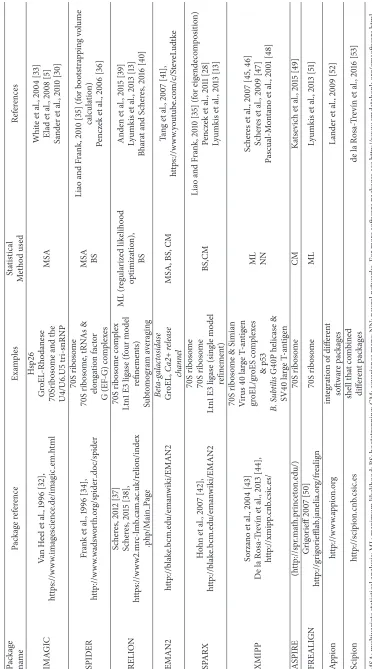
There are many techniques that can be used in the analysis of heterogeneous data; however, each biological dataset will often require a very specific method to resolve the problem. The different statistical methods, examples of which have already been described, are often used in conjunction with each other (Table 1). Pe˜na with collaborators [111] used the ML method and a NN self-organizing map to align and classify the dataset of the full-length hexameric TrwK, a VirB4 homologue, in the conjugative plasmid R388. This

molecule consists of two rings, one with a diameter of 132 ˚A

corresponding to the N-terminal region of the protein and

one with a diameter of 124 ˚A from the C-terminal region.

Pascual-Montano et al., 2001 [48], also used ML classifica-tion and NN (SOM) to look at the variability of negative stain

images of the G40P helicase ofBacillus subtilisbacteriophage

SPP1 and cryoelectron images of the Simian Polyomavirus SV40 large T-antigen. This combination of approaches (ML and SOM) used power spectra to determine symmetry of G40P particle images and has demonstrated the presence of three types of particles, one with 4-fold symmetry and another with 5-fold symmetry and asymmetric particles possibly which were not very well aligned. Analysis of results has suggested that images belonging to the asymmetric group should be removed completely from the data for further analysis. Using the techniques mentioned above the images of the SV40 large T-antigen revealed the existence of several classes of particles. Some of these particles exhibit axial curvature along the major vertical axis.

When E1 helicase was labelled with FAB antibodies, only about 30% of the particles had antibody bound to it. It was difficult to see any differences in images since the intensities related to the FAB were minimal. To overcome this problem a 3D bootstrapping technique was employed in combination with 3D MSA [112]. The first 10 eigenvectors demonstrate the variations of density distribution in the area of the FAB position.

The existence of many different software packages pro-vides a variety of options to electron microscopists for analysis of their data (Table 1, [102, 113–117]). The packages only partly overlap and it would be useful to combine the best features of each software program. But these packages have different data formats; for example, the output file from IMAGIC needs to be converted into SPIDER format prior to the use of that program. Therefore one should take care of the data consistency between the packages. Nowadays there are several packages (EMAN2, IMAGIC, BSOFT, and some others) that can do that easily.

EM is presently obtaining structures at high resolution on a regular basis. Increasing computational power and multiprocessor technology allows millions of images to be processed. Biocomplexes in solution naturally have different conformational states and these are all captured at the same time during cryo-EM imaging. The presence of heterogeneity means that higher resolution features could be averaged out during the reconstruction phase. To avoid this problem we need to take care of “computational purification” of the entire dataset and hence the separation of data is required into more

homogeneous subsets. Researchers are constantly developing new computational techniques for sorting heterogeneous datasets and extending the current approaches to more com-plex problems. Accurate structure determination is impor-tant in understanding the structure/function relationship of biological processes. Biological processes are not static but the components are in constant natural motion. Therefore, to understand the interactions, their sequence, and how they can be controlled, especially in the case of diseases, we need to capture different conformational states of biocomplexes. Consequently, much data collected now is heterogeneous and the methods described here as well as their applications are becoming increasingly significant. Table 1 lists some of the packages available, the methods implemented in them, and some examples of their usage. The reader has to take into consideration that it is difficult to provide a complete overview of all methods presently developed, but we hope to provide the readers with a starting point for their analysis and the ability to extend the approaches they use to obtain accurate final structures.

Disclosure

Current address for D. K. Clare is as follows: Diamond Light Source Ltd., Diamond House, Harwell Science and Innovation Campus, Didcot, Oxfordshire OX11 0DE.

Competing Interests

The authors declare that they have no competing interests.

Acknowledgments

The authors would like to thank D. Houldershaw for com-puter support and Abid Javed for the preparation of figures. The work of A. Ignatiou is supported by a Biotechnology and Biochemical Sciences Research Studentship (LiDO) and that of E. V. Orlova by a Biotechnology and Biochemical Sciences Research Council Grant BB/J008648/1, MRC MR/K012401/1, and Welcome Trust 101488/Z/13/Z.

References

[1] W. R. Wikoff, J. F. Conway, J. Tang et al., “Time-resolved molecular dynamics of bacteriophage HK97 capsid maturation interpreted by electron cryo-microscopy and X-ray crystallog-raphy,”Journal of Structural Biology, vol. 153, no. 3, pp. 300–306, 2006.

[2] S. C. Blanchard, H. D. Kim, R. L. Gonzalez Jr., J. D. Puglisi, and S. Chu, “tRNA dynamics on the ribosome during translation,”

Proceedings of the National Academy of Sciences of the United States of America, vol. 101, no. 35, pp. 12893–12898, 2004. [3] P. V. Cornish, D. N. Ermolenko, H. F. Noller, and T. Ha,

“Spon-taneous intersubunit rotation in single ribosomes,”Molecular Cell, vol. 30, no. 5, pp. 578–588, 2008.