BIROn - Birkbeck Institutional Research Online
Zhang, X. and Hu, W. and Xie, N. and Bao, H. and Maybank, Stephen
J. (2015) A robust tracking system for low frame rate video. International
Journal of Computer Vision 115 (3), pp. 279-304. ISSN 0920-5691.
Downloaded from:
Usage Guidelines:
Please refer to usage guidelines at
or alternatively
A Robust Tracking System for Low Frame Rate Video
Xiaoqin Zhang1 · Weiming Hu2 · Nianhua Xie2 · Hujun Bao3 · Stephen Maybank4
Received: 17 April 2013 / Accepted: 18 March 2015 © Springer Science+Business Media New York 2015
Abstract Tracking in low frame rate (LFR) videos is one of the most important problems in the tracking literature. Most existing approaches treat LFR video tracking as an abrupt motion tracking problem. However, in LFR video tracking applications, LFR not only causes abrupt motions, but also large appearance changes of objects because the objects’ poses and the illumination may undergo large changes from one frame to the next. This adds extra difficulties to LFR video tracking. In this paper, we propose a robust and general tracking system for LFR videos. The tracking system con-sists of four major parts: dominant color-spatial based object representation, bin-ratio based similarity measure, annealed
Communicated by M. Hebert.
B
Xiaoqin ZhangWeiming Hu [email protected]
Nianhua Xie [email protected]
Hujun Bao [email protected]
Stephen Maybank [email protected]
1 Institute of Intelligent System and Decision, Wenzhou
University, Zhejiang, China
2 National Laboratory of Pattern Recognition, Institute of
Automation, Chinese Academy of Sciences, Beijing, China
3 Department of Computer Science, Zhejiang University,
Zhejiang, China
4 Department of Computer Science and Information Systems,
Birkbeck College, London, UK
particle swarm optimization (PSO) based searching, and an integral image based parameter calculation. The first two parts are combined to provide a good solution to the appear-ance changes, and the abrupt motion is effectively captured by the annealed PSO based searching. Moreover, an integral image of model parameters is constructed, which provides a look-up table for parameters calculation. This greatly reduces the computational load. Experimental results demonstrate that the proposed tracking system can effectively tackle the difficulties caused by LFR.
Keywords Low frame rate·Tracking·Dominant color· Bin-ratio matching metric·Particle swarm optimization
1 Introduction
Tracking in LFR videos has received more and more attention because of its wide applications in micro embedded systems (e.g. mobile vision systems and car vision systems) and visual surveillance. There are two major situations in which LFR videos are produced: (1) LFR videos may be produced when image frames are missed because of hardware delay in the image acquisition system or the limitation of transmission bandwidth; (2) the frame rate of the data streams may be down-sampled because of limitations in the storage or the processing power of the CPU. The design of robust tracking systems for LFR videos is an important and challenging issue in the tracking literature.
frames are small. In typical applications of particle filter-ing to trackfilter-ing (Isard and Blake 1998), motion prediction is based on the tracking results in the previous frame. For the iterative optimization based tracking algorithms, such as
Kanade–Lucas–Tomasi (KLT) (Tomasi and Kanade 1991),
template matching algorithm (Hager and Belhumeur 1998) and mean shift (Comaniciu et al. 2003), the initialization of the optimizer is based on the tracking results in the previ-ous frame. So the above classical tracking algorithms do not yield satisfactory results when applied to LFR video.
Tracking in LFR videos has been much less investigated than tracking in full frame rate videos. Porikli and Tuzel
(2005, 2006), extend the mean shift algorithm to a multi-kernel mean shift algorithm, and apply it to the motion map which is obtained from background subtraction, in order to overcome the abrupt motion caused by LFR video. A cas-cade particle filter which integrates conventional tracking and detection is proposed byLi et al.(2008) for LFR video track-ing. In this approach, detectors learned from different ranges of samples are adopted to detect the moving object. This approach requires complex detectors and time-consuming off-line training, and the detectors only work well in face tracking. InCarrano (2009), the object motion is detected from background subtraction, and then four features, namely phase cross correlation, average intensity difference, velocity difference, and angle difference are combined for match-ing between consecutive image frames.Zhang et al.(2009) adopt region based image differencing to estimate the object motion. The predicted motion is used to guide the particle propagation in a particle filter. In summary, all of the above work assumes that the only problem with LFR tracking is abrupt motion. However, in practice, LFR not only causes abrupt motion, but also large appearance changes because the object pose and the illumination may undergo large changes from one frame to the next. As a result, it is necessary to take both the abrupt motion and the appearance changes of the object into consideration. In order to design a robust track-ing system for LFR videos, we start with the followtrack-ing two requirements: (1) robust appearance modeling, to deal with the changes in object pose and illumination; (2) effective searching methods, to capture the abrupt motion of the object. Below, we will investigate the related work on appearance modeling and motion searching.
1.1 Related Work
1.1.1 Appearance Model
The appearance model of the object is a basic issue to be considered in tracking algorithms. An image patch model (Hager and Belhumeur 1998), which takes the set of pix-els in the target region as the model representation, is a direct way to model the target, but it loses the
discrimina-tive information that is contained in the pixel values. The color histogramComaniciu et al. (2003),Nummiaro et al.
(2003) provides global statistical information about the tar-get region which is robust to noise, but it has two major problems: (1) the histogram is very sensitive to illumina-tion changes; (2) the relative posiillumina-tions of the pixels in the image are ignored. A consequence of (2) is that trackers based on color histograms are prone to lose track if the object is near to other objects with a similar appearance. InIsard and Blake(1998), curves or splines are used to represent the apparent boundary of the object, and the Condensation algo-rithm is developed for contour-based tracking. Due to the simplistic representation, which is confined to the apparent boundary, the algorithm is sensitive to image noise, leading to tracking failures in cluttered backgrounds.Stauffer and Grimson(1999) employ a Gaussian mixture model (GMM) to represent and recover the appearance changes in consec-utive frames.Jepson et al.(2003) develop a more elaborate Gaussian mixture model which consists of three components
S,W,L, where theS component models temporally stable images, theW component models the two-frame variations, and theLcomponent models data outliers, for example those caused by occlusion. An online EM algorithm is employed to explicitly model appearance changes during tracking. Later,
Zhou et al.(2004) replace the componentL with a compo-nentF, which is a fixed template of the target, to prevent the tracker from drifting away from the target. This appearance based adaptive model is embedded into a particle filter to achieve robust visual tracking.Wang et al.(2007) present an adaptive appearance model based on a mixture of Gaussians model in a joint spatial-color space, referred to as SMOG. SMOG captures rich spatial layout and color information. However, these GMM based appearance models consider each pixel independently and with the same level of con-fidence, which is not reasonable in practice. InPorikli et al.
(2006), the object to be tracked is represented by a covari-ance descriptor which enables efficient fusion of different types of features and modalities. Another category of appear-ance models is based on subspace learning. For example, in
However, the aforementioned appearance models ignore the background information and do not perform well when the background is noisy and cluttered. In order to deal with these cases, a set of discriminative based appearance models are proposed (Collins et al. 2005;Lin et al. 2004; Avidan 2004;Avidan 2007;Grabner et al. 2006;Grabner et al. 2008;
Saffari et al. 2010;Babenko et al. 2011). For example,Collins et al.(2005) firstly note the importance of background infor-mation for object tracking, and formulate tracking as a binary classification problem between the tracked object and its sur-rounding background. InLin et al.(2004), a two-class Fisher discriminant analysis (FDA) based model is proposed to learn a discriminative subspace to separate the object from the background. InAvidan(2007), an ensemble of online weak classifiers are combined into a strong classifier. A proba-bility map is constructed by the classifier to represent the probabilities of the pixels belonging to the object or the back-ground.Grabner et al.(2006) adopt online boosting to select discriminative local tracking features. Each selected feature corresponds to a weak classifier that separates the object from the background.Saffari et al.(2010) introduce a novel on-line random forest algorithm for feature selection that allows for on-line building of decision trees. InBabenko et al.(2011), Babenko et al. use multiple instance learning instead of tradi-tional supervised learning to learn the weak classifiers. This strategy is more robust to the drifting problem.
Overall, the complex appearance models (such as the sub-space model, the Gaussian mixture model and learning based appearance models) do not adapt well to the large appearance changes, while the simple models (such as color histogram) are not robust and discriminative enough. Since there are large appearance changes of the object in LFR video, it is necessary to find a balance between adaptability and robust-ness.
1.1.2 Searching Method
Most of the existing tracking algorithms can be formulated as optimization processes, which are typically tackled using either deterministic searching methods (Kass et al. 1988;
Hager and Belhumeur 1998;Comaniciu et al. 2003) or sto-chastic searching methods (Isard and Blake 1998;Nummiaro et al. 2003;Bray et al. 2007). Deterministic searching meth-ods usually involve a gradient descent search to minimize a cost function. The snakes model introduced byKass et al.
(1988) is a good example. The aim is to obtain a tight con-tour enclosing the object by minimizing an energy function. InHager and Belhumeur(1998), the cost function is defined as the sum of squared differences between the observation candidate and a fixed template. Then the motion parameters are found by minimizing the cost function through a gra-dient descent search. Mean shift, which firstly appeared in
Fukunaga and Hostetler(1975) as an approach for estimating
the gradient of a density function, is applied byComaniciu et al. (2003) to visual tracking, in which the cost function between two color histograms is minimized through the mean shift iterations. In general, deterministic searching methods are usually computationally efficient but they easily become trapped in local minima. In contrast, stochastic searching methods have a higher probability of reaching the global optimum of the cost function. For example, in Isard and Blake (1998), Nummiaro et al. (2003), object tracking is viewed as an online Bayesian inference problem, which is solved by randomly generating a large number of particles to find the maximum of the posterior distribution.Bray et al.
(2007) use the stochastic meta-descent strategy to adapt the step size of the gradient descent search, and thus avoid local minima of the optimization process, when applied to articu-lated structure tracking.Leung and Gong(2007) incorporate random subsampling into mean shift tracking to boost its effi-ciency and robustness for low-resolution video sequences. Compared with the deterministic counterparts, stochastic searching methods are usually more robust, but they incur a large computational load, especially if the state space has a high dimension.
As stated in Sect.1, both the deterministic searching meth-ods and stochastic searching methmeth-ods are based on the state continuity hypothesis in tracking applications. For this rea-son, they do not yield satisfactory results in case of LFR video.
1.2 Our Work
In view of the forgoing discussions, we analyze the track-ing problem in case of LFR video from the followtrack-ing three aspects: (1) object representation, (2) matching criterion, (3) searching method, and design a robust and general track-ing system for LFR video. Although our tracktrack-ing system is designed with the LFR video in mind, it can handle the sim-ilar tracking problems in the normal video arising from fast moving objects or camera motion. The main contributions of our work are:
1. The object is represented by the dominant color-spatial distribution of the object region. This representation can extract the dominant color modes of the object region, and simultaneously remove the noisy image pixels. In addition, the spatial distribution of the dominant color mode is utilized to improve the discriminative ability of the representation.
Fig. 1 The flow chart of the proposed tracking system
3. In order to handle the abrupt motions caused by LFR video, we propose an annealed particle swarm opti-mization (PSO) method. Inspired by the social behavior of bird flocking, the particles in this searching method cooperate and communicate with each other, and the shared information guides the evolution of the particles. This mechanism realizes robust searching for the abrupt motions.
4. Each particle specifies a candidate image region. The fitness value of a particle is evaluated during the PSO iter-ation process, using the similarity between the candidate image region and the object template. Many candidate image regions may overlap, and the image pixels inside the overlapping region will be used in many separate cal-culations of the similarity between the candidate image region and the object template. This involves a large and unnecessary computational load. In order to avoid the unnecessary computation, we calculate a integral image of model parameters which establishes a parameter-particle look-up table. In this way, each pixel inside the candidate region needs to be calculated only once. As a result, the computational complexity is greatly reduced.
An overview of the proposed tracking system for LFR video is systematically presented in Fig.1. There are four major components in the proposed tracking system: (1) dom-inant color-spatial based object representation, (2) bin-ratio based similarity measure, (3) integral image of model para-meters, (4) annealed PSO based searching process. We will give a detailed description of each component in the follow-ing sections.
The rest of the paper is organized as follows. The dominant color-spatial based object representation is described in Sect.
2. The bin-ratio based similarity measure is introduced in Sect.3. The annealed PSO searching method and integral image of model parameters are presented in Sects.4and5
respectively. Experimental results are shown in Sects.6and
7is devoted to conclusion.
2 Dominant Color-Spatial Based Object
Representation
In our work, the major color modes inside the object region are firstly obtained by a dominant-set based clustering
algo-rithm, and then the spatial distribution of each color mode is extracted to enhance the discriminative ability of the color model.
2.1 Dominant-Set Based Clustering Algorithm
Suppose given an undirected edge-weighted graph G =
(V,E,A), where V is the vertex set, E is set of weighted edges that link different vertices, andAis a symmetric simi-larity matrix in whichai jrepresents the similarities between vertexi and vertex j. The aim of dominant-set clustering is to cluster the vertices in V according to the similarity matrix A. Concepts and algorithms for dominant-set clus-tering are briefly introduced hereinafter for the convenience of the reader.
2.1.1 Concept of Dominant Set
A dominant set, as defined byPavan and Pelillo(2003), is a combinatorial concept in graph theory that generalizes the notion of a maximal complete subgraph to edge-weighted graphs. The characteristics of dominant-set clustering rest with the definition of dominant sets.
Specifically, letS ⊆V be a nonempty subset of vertices. For any vertexi ∈S, the average weighted degree ofirelative toSis defined as
DS(i)= 1
|S|
j∈S
ai j (1)
where|S|is the number of vertices inS. For a vertex j ∈/ S, the similarityφS(i,j)between verticesiand j relative toS is defined asφS(i,j)=ai j−DS(i). Then, the weightwS(i) ofi ∈Srelative toSis defined as
wS(i)=
1, if |S| =1
j∈S\{i}φS\{i}(j,i)wS\{i}(j), otherwise (2)
W(S)=
i∈S
wS(i) (3)
The setS is defined as a dominant set if it satisfies the fol-lowing conditions (Pavan and Pelillo 2003): (1) ∀T ⊂ S,
W(T) > 0; (2) ∀i ∈ S, wS(i) > 0; and (3) ∀i ∈/ S, wS(i) <0. Condition (1) indicates that vertices in each sub-set ofSare closely and firmly united. Condition (2) indicates thatShas large attraction to each vertex inS. Condition (3) indicates thatShas no large attraction to any vertex outside
S. Conditions (1) and (2) describe the internal homogeneity ofS. Condition (3) describes the external heterogeneity ofS. The definition of a dominant set simultaneously emphasizes internal homogeneity and external inhomogeneity, and thus is considered to be a general definition of “cluster”.
2.1.2 Clustering Algorithm
Pavan and Pelillo(2003) establish an intriguing connection between the dominant set and a quadratic optimization prob-lem as follows:
maximize g(z)=zTAz
subject to z∈ (4)
wherezis the indictor vector of samples in the clustering process that satisfies
=
z∈Rn:zi ≥0 and n
i=1
zi =1
.
Ais the similarity matrix of the input samples, andg(·)is the objective function which defines the cohesiveness of a cluster in a natural way. Letz∗denote a strict local solution of (4), and letσ(z∗)be the vertex support set ofz∗:σ (z∗)= {i|z∗i >0}. It has been proved inPavan and Pelillo(2003) that the vertex support setσ(z∗)corresponds to a dominant set in the graph represented by A. This allows us to formulate the pairwise clustering problem as the problem of finding a vectorz∗that solves (4). The valueg(z∗)at the local maximum indicates the “cohesiveness” of the dominant-set cluster specified by
z∗.
Pavan and Pelillo(2003) use the following iterative equa-tion to solve (4)
zi(t+1)=zi(t) (
Az(t))i
z(t)TAz(t), i =1, . . . ,n (5)
where t indexes the number of iterations. Meanwhile, the authors provePavan and Pelillo(2003) that the trajectoryz(t)
[image:6.595.307.545.101.204.2]generated by Eq. (5) converges to a strict local maximizer of program (4).
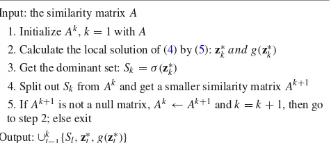
Table 1 Dominant-set clustering algorithm
Input: the similarity matrixA
1. InitializeAk,k=1 withA
2. Calculate the local solution of (4) by (5):z∗kand g(z∗k)
3. Get the dominant set:Sk=σ(z∗k)
4. Split outSkfromAkand get a smaller similarity matrixAk+1
5. IfAk+1is not a null matrix,Ak←Ak+1andk=k+1, then go to step 2; else exit
Output:∪kl=1{Sl,z∗l,g(z∗l)}
Based on the above discussion, dominant set clustering can be conducted in a bipartition way. To cluster the samples, a dominant set of the weighted graph is found by Eqs. (4) and (5) and then removed from the graph. This process is iterated until the graph is empty. Each dominant set defines a clus-ter. Table1contains the algorithm for the clustering process. Therefore, dominant-set clustering has two advantages: (1) In contrast with many traditional clustering algorithms (k-means and mean shift), it can automatically determine the number of the clusters; (2) the computational demand is low compared with that of other graph-theoretic clustering algo-rithms that rely on an eigen analysis ofA.
2.1.3 Fast Assignment Algorithm
To group any new samples obtained after the clustering process has taken place,Pavan and Pelillo(2005) propose a fast assignment algorithm which does not need to conduct a new dominant-set clustering. Let S ⊂ V be a subset of vertices which is dominant in the original graphG and let
i be a new data vertex. As stated in Sect.2.1.1, the sign of
wS∪{i}(i)provides an indication as to whetheriis tightly or loosely coupled with the vertices inS. However, if only the sign ofwS∪{i}(i)is considered, then the same point can be assigned to more than one class. This ambiguity is removed as follows. The degree of participation ofiinS∪ {i}is given by the ratio betweenwS∪{i}(i)andW(S∪ {i}). Since com-puting the exact value of the ratiowS∪{i}(i)/W(S∪ {i})is computationally expensive, a simple approximation formu-las is provided inPavan and Pelillo(2005).
wS∪{i}(i)
W(S∪ {i}) ≈
|S| −1
|S| +1
αTz∗
S
g(z∗S)−1
(6)
where α is an affinity vector containing the similarities between the new sampleiand the originalnsamples, andz∗S
Table 2 Dominant-set fast assignment algorithm
Input: Affinity vectorα∈Rn,∪kl=1{Sl,z∗l,g(zl∗)}
1. Computebl=||SSll|−|+11(α
Tz∗ l
g(z∗l)−1),l∈ {1, . . . ,k} 2.l∗=argmaxlbl
3. Ifbl∗>0, assignαto the clusterSl∗; elsel∗=0,αis consider as
an outlier Output:l∗
2.2 Dominant Color Mode Extraction
Given a image region, we first convert theRGBcolor space to thergIspace using the following formulas:
r =R/(R+G+B), g=G/(R+G+B), I =(R+G+B)/3
Then we define the pixel-pairwise graph, where the weight
ai j on the edge connecting nodei and node j is calculated by:1
ai j =cexp(−||fi −fj||2) (7)
wherefi = (r,g,I)is the intensity value of pixeli in the
rgIcolor space, andcis the normalization factor. Then, we apply the dominant set based clustering algorithm to the con-structed pixel-pairwise graph, and obtain the dominant color modes{Sl,zl}kl=1. In tracking applications, if all the pixels are clustered by a dominant set based clustering algorithm, then there will be many small clusters. Therefore the cluster-ing is stopped if the number of the remaincluster-ing pixels (vertices) is less than 5 % of the total pixel number inside the object region. This criterion has two advantages: (1) the outliers can be effectively filtered out; (2) the number of dominant colors is not strongly affected by the size of the object.
2.3 Spatial Layout of the Dominant Color
The above dominant color based representation captures the color distribution in the image region of interest. However, the spatial layout of pixels falling into the same color mode is ignored. In order to overcome this problem, the spatial mean
μland the variancelof thelth color mode are extracted as follows.
μl =
ipiδ(L(i)−l)
iδ(L(i)−l)
(8)
l =
i(pi−μl)(pi−μl)Tδ(L(i)−l) iδ(L(i)−l)
(9)
1Here, the componentIis normalized asI/255.
wherepiis the coordinate of the pixelirelative to the center position of the image region, andL(i)is a label function to assign the pixeli to a given cluster.δ(·)is the Kronecker function such thatδ(L(i)−l)=1 ifL(i)=landδ(L(i)− l)=0 otherwise.
As a result, the image region of interest can be represented by{ωl,μl,l}lk=1, whereωlis the weight of thelth dominant color mode and is calculated as follows:
ωl=
iδ(L(i)−l)
k l=1
iδ(L(i)−l)
(10)
3 Similarity Measure for Matching
3.1 Bin-Ratio Based Color Distance Measure
3.1.1 Motivation
Let uO = {ulO}kl=1 be a k-bin color histogram that rep-resents the color distribution of the pixels in the object template. The candidate histogramuC = {uCl }lk=1is calcu-lated as follows: first, the pixels inside the candidate image patch are assigned to the bins of the object histogramuO
using the fast assignment algorithm in Table 2, and then
uC is obtained according to the results of the assignment. Traditionally, the similarity between uO = {ulO}kl=1 and
uC = {uCl }kl=1is evaluated by the Bhattacharyya measure
Comaniciu et al.(2003):ρ(uO,uC)=lk=1 uOl ulC, or the histogram intersection measureSwain and Ballard(1991):
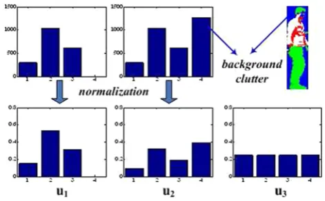
Q(uO,uC)=lk=1min(ulO,ulC). However, these measures are sensitive to illumination changes and image clutter. In tracking applications, as the object region is often represented by a rectangle, the histograms are often corrupted by back-ground clutter that is irrelevant to the object. For example, as shown in Fig.2, a large portion of pixels represented with blue
Fig. 2 An example of background clutter problem (u1: histogram
without background pixels,u2: histogram with background pixels,u3:
[image:7.595.306.542.556.702.2]are background, which fall into the fourth bin of histogram. We can see thatu1andu2look very different after
normal-ization, which means pixels from the background introduce noise into the histogram which may cause inaccurate match-ing.
To validate the above claim, we test the above two mea-sures on this example. By introducing a uniformly distributed histogramu3for reference, the following results are obtained:
ρ(u1,u2)=0.24< ρ(u1,u3)=0.25,Q(u1,u2)=0.6<
Q(u1,u3) = 0.65. Both ρ(·,·) and Q(·,·) are similarity
measures which means they can not find a correct match amongu1,u2andu3in this case.
3.1.2 Proposed Distance Measure
To overcome these drawbacks, we introduce a bin-ratio based color distance measure, which was firstly proposed for cate-gory and scene classification in our previous workXie et al.
(2010). For ak-bin histogramu= {ul}kl=1, ak∗kratio matrix Br is defined using the ratios of paired bin values. Each ele-ment in the matrix has the form(ui/uj)which measures the ratio of biniand j. The ratio matrix is shown as follows:
Br =
ui
uj
i,j
= ⎡ ⎢ ⎢ ⎢ ⎢ ⎢ ⎣ u1 u1 u2
u1 · · ·
uk u1
u1
u2
u2
u2 · · ·
uk u2 · · · · u1 uk u2
uk · · · uk uk ⎤ ⎥ ⎥ ⎥ ⎥ ⎥ ⎦ (11)
With the definition of the ratio matrix, we compare the
vth bin between two histogramsuO anduC using the dis-tance measureMv, which is defined as the sum of squared difference between thevth rows of the corresponding ratio
matrices ofuOanduC:kl=1
ulO uO
v − uCl uC v
2
. The ratio matrix
Br suffers from the instability problem when its entries are close to zero. To avoid this problem, we include the nor-malization part u1O
v +
1 uC
v and define the following distance measure,
Mv(uO,uC)=
k
l=1
ulO uO
v −
uCl uC v / 1 uO v + 1 uC v 2 = k
l=1
ulOuCv −uvOuCl uO
v +uCv
2
(12)
As shown in Eq. (12), the numeratorulOuvC−uOvulCcan still represent the difference of ratios. The denominatoruvO+uCv is similar to the normalization part in theX2distancePuzicha et al.(1997), included to make the distance measure more
stable. Based on the L2 normalization k
l=1u2l = 1, the above distance measure can be simplified as follows.
Mv(uO,uC)= k
l=1
ulOuCv −uOvuCl uO
v +uCv
2
=
k
l=1((uCvulO)2+(uvOulC)2−2uOvuCvulOuCl) (uO
v +uCv)2
=(uCv)2
k
l=1(uOl )2+(uvO)2
k
l=1(ulC)2−2uvOuCv
k
l=1(ulOuCl) (uO
v +uCv)2
=(uCv)2+(uvO)2−2uvOuCv
k
l=1(ulOuCl) (uO
v +uCv)2
=(uCv +uvO)2−uOvuCv(2+
k
l=12ulOuCl) (uO
v +uCv)2
=(uCv +uvO)2−uOvuCv
k
l=1((uOl )2+(ulC)2+2uOl uCl) (uO
v +uCv)2
=(uCv +uvO)2−uOvuCv
k
l=1(ulO+uCl)2 (uO
v +uCv)2
=1− u
O
vuCv
(uO
v +uCv)2||
uO+uC||22
where||uO +uC||2is theL2norm ofuO+uCand can be
obtained before the distance calculation. Therefore, this dis-tance measure has a linear computational complexity in the bin number, as do the Bhattacharyya distance and histogram intersection distance.
The bin-ratio distance between color histogramsuO and
uCis formulated as follows:
c(uO,uC)= k
v=1
Mv(uO,uC)
=
k
v=1
1− u
O
vuCv (uO
v +uCv)2||u
O +
uC||22
(13)
The above bin-ratio distance measure is robust under 1) illu-mination changes, 2) partial occlusion, 3) contaillu-mination by background pixels. For the example in Fig. 2, the result of the bin-ratio distance measure is c(u1,u2) = 1.4 <
c(u1,u3)=1.5 which is correct. These claims are further
supported by experiments on both synthetic data and real data as reported in Sect.6.
3.2 Spatial Distance Measure
For the object image and a candidate region, the spa-tial mean and the covariance matrix of each color mode are computed as in Eqs. (8) and (9) accordingly:{μlO,lO}kl=1,
{μC
l ,Cl }lk=1. Together with the weight of the
correspond-ing color mode, the spatial distance measures(uO,uC)is defined as follows:
s(uO,uC)= k
l=1
ωlexp
−1
2(μ O l −μ
C l )
T(O l
+C
l )−1(μlO−μCl )
(14)
where the weightωl is calculated using the target template as in (10), and updated in the parameter updating process.
As a result, the dominant color-spatial based similarity measure can be defined as follows.
cs(uO,uC)=exp
1
2σ12(1−s(u O,uC))
∗exp
− 1
2σ22c(u O,
uC)
(15)
whereσ12, σ22are the parameters which balance the influence of spatial distance and bin-ratio distance.
3.3 Parameter Updating
In most tracking applications, the tracker must deal with changes in the appearance of the object, so it is necessary to design an updating scheme for the parameters employed in the appearance model.
The updating process is described in detail as follows.
1. Suppose the tracking result for the current frame has been obtained. Based on the label information and the positions of the pixels inside the image region obtained by tracking results, the parameters{ωl,μl,l}kl=1of the
object model are updated as in Eqs. (8), (9) and (10). 2. There may be outlier pixels left inside the image region
obtained by tracking results when applying the dominant-set fast assignment algorithm to the image region. If the number of the outlier pixels exceeds 1/6 of the total number of pixels inside the tracked image region and their cohesiveness value evaluated byg(·)exceeds the cohesiveness value of the smallest cluster in the target template, then these pixels are grouped as a new clus-ter which is added to the object model; otherwise these pixels are filtered out as noise.
In this way, the parameter updating process makes a trade-off between robustness and adaptation. As a result, it not
only effectively captures the variations of the target, but also reliably prevents drifting during tracking.
4 Swarm Intelligence Based Searching Method
The abrupt motions in LFR image sequences cause sample impoverishment when they are tracked using a particle filter. We first investigate the reason for this sample impoverish-ment and then propose a swarm intelligence based searching method: annealed particle swarm optimization, which can overcome the sample impoverishment problem both in the-ory and practice.
4.1 Sample Impoverishment Problem of Particle Filter
The particle filter is an on-line Bayesian inference process for estimating an unknown statest at timet from sequential observationso1:tperturbed by noise. The Bayesian inference process is based on
p(st|o1:t)∝ p(ot|st)p(st|o1:t−1) (16)
where the priorp(st|o1:t−1)is the propagation of the previous
posterior density along the temporal axis,
p(st|o1:t−1)=
p(st|st−1)p(st−1|o1:t−1)dst−1 (17)
When the state transition distribution p(st|st−1)and
obser-vation distribution p(ot|st) are non-Gaussian, the above integration is intractable and one has to resort to numeri-cal approximations such as particle filters. The basic idea of particle filter is to use a number of particles{sit}iN=1, sampled from the state space, to approximate the posterior distribu-tion by p(st|o1:t) = N1 iN=1δ(st −sit), whereδ(·)is the Dirac function. Since it is usually impossible to sample from the true posterior, an easy-to-implement distribution, the so-called proposal distributiondenoted by q(·) is employed, hencesit ∼q(st|sit−1,o1:t), (i =1, . . . ,N), and each parti-cle’s weight is set to
ηi t ∝
p(ot|sit)p(sit|sit−1)
q(st|sit−1,o1:t)
. (18)
Finally, the posterior probability distribution is approximated byp(st|o1:t)=
N
i=1ηitδ(st−sit).
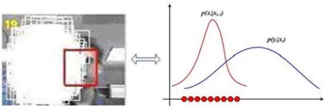
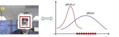
The proposal distributionq(·)is critically important for a successful particle filter because it concerns putting the sampling particles in the useful areas where the posterior is significant. In tracking applications, the state transition distri-butionp(st|st−1)is usually taken as the proposal distribution
Fig. 3 Sample impoverishment problem
most state transition models use a naive random walk around the previous system state. As shown in Fig.3, when the object undergoes abrupt motion, the performance of the particle fil-ter is very poor because most particles have low weights, thereby leading to the well-known sample impoverishment problem.
As proved inDoucet et al.(2000), it is shown that the ‘opti-mal’ importance proposal distribution isp(st|sit−1,ot)in the sense of minimizing the variance of the importance weights. However, in practice, it is impossible to usep(st|sit−1,ot)as the proposal distribution in the non-linear and non-Gaussian cases, because it is difficult to sample from p(st|sit−1,ot) and to evaluate p(ot|sit−1) =
p(ot|st) p(st|sit−1)dst. So the question is, how to incorporate the current observationot into the transition distributionp(st|st−1)to form an effective
proposal distribution at a reasonable computation cost?
4.2 Annealed Particle Swarm Optimization
In this part, we propose an annealed particle swarm optimiza-tion (APSO) algorithm to effectively search for the object motion parameters. From the particle filtering point of view, the searching process in APSO is an approximation to the optimal importance sampling.
4.2.1 Iteration Process
Particle swarm optimizationKennedy and Eberhart(1995), is a population-based stochastic optimization technique, which is inspired by the social behavior of birds flocking. In detail, a PSO algorithm is initialized with a group of random particles
{si,0}iN=1(Nis the number of particles). Each particlesi,0has a corresponding fitness value f(si,0)and a relevant velocity
vi,0, which is a function of the best state found by that particle (pi, for individual best), and of the best state found so far among all particles (g, for global best). Given these two best values, the particle updates its velocity and state with the following equations in thenth iteration,
vi,n+1=ξnvi,n+ϕ1ρ1(pi−si,n)+ϕ2ρ2(g−si,n) (19) si,n+1=si,n+vi,n+1 (20)
where ξnis the inertial weight, the ϕ1, ϕ2 are acceleration
constants, andρ1, ρ2∈(0,1)are uniformly distributed
ran-dom numbers. The inertial weightξnis usually a monoton-ically decreasing function of the iteration number n. For example, given a user-specified maximum weightξmax , a minimum weightξmi n and the initialization ofξ0 = ξmax, one way to updateξnis as follows:
ξn+1=ξn−dξ, dξ =(ξ
max−ξmi n)/nmax (21)
wherenmax is the maximum iteration number.
In order to reduce the number of parameters in the above PSO iteration process, we propose an annealed Gaussian ver-sion of PSO algorithm (APSO), in which the iteration process is modified as follows:
vi,n+1= |r1|(pi−si,n)+ |r2|(g−si,n)+ (22) si,n+1=si,n+vi,n+1 (23)
where|r1|and|r2|are the absolute values of the independent
samples from the Gaussian probability distributionN(0,1), andis a zero-mean Gaussian perturbation noise which pre-vents the particles from becoming trapped in local optima. The covariance matrix ofis changed in an adaptive simu-lated annealing wayIngber(1993):
=e−cn (24)
whereis the covariance matrix of the predefined transition distribution,cis an annealing constant, andnis the iteration number. The elements indecrease rapidly as the iteration numbernincreases which enables a fast convergence rate.
Then the fitness value of each particle is evaluated using the observation model p(oi,n+1|si,n+1)as follows.
f(si,n+1)= p(oi,n+1|si,n+1) (25)
Here, the observation modelp(oi,n+1|si,n+1)reflects the
sim-ilarity between the candidate image observationoi,n+1and the target model which is defined in Eq. (15).
After the fitness value of each particle f(si,n+1)is
evalu-ated, the individual best and the global best of particles are updated in the following equations:
pi =
si,n+1,if f(si,n+1) > f(pi)
pi, else (26)
g=arg max
pi f(p i)
(27)
[image:10.595.53.288.81.160.2]As a result, the particles interact locally with one another and with their environment in analogy with the ‘cognitive’ and ‘social’ aspects of animal populations, and eventually cluster in the regions where the local optima of f(·)are located. In Eq. (22), the three terms on the right hand side representcognitive effect,social effectand noise part respec-tively, wherecognitive effectrefers to the evolution of the particle according to its own observations, andsocial effect
refers to the evolution of the particle according to the coop-eration between all particles.
4.2.2 Approximation to Optimal Importance Sampling
When applied to the tracking applications, the sequential information should be incorporated into the annealed PSO algorithm. In particular, the initial particles in the annealed PSO algorithm are firstly sampled from the transition distri-bution as follows:
sit,0∼N(pit−1,) (28)
In our tracking process, resampling is not needed because the individual best of the particle set{pit−1}Ni=1converged at time
t−1 provides a compact sample set for time propagation, and then the annealed PSO iterations are carried out until convergence.
From the particle filtering point of view, the above process is a two-stage sampling strategy to generate samples that approximate to samples from the ‘optimal’ proposal distrib-utionp(st|sit−1,ot): first, in the coarse importance sampling stage, the particles are sampled from the state transition distribution as in (28) to enhance their diversity. In the fine importance sampling stage, the particles evolve through APSO iterations, and are updated according to the newest observations. In fact, this is essentially a latent multi-layer importance sampling process with an implicit proposal dis-tribution. Letst ∈ Rdbe ad-dimensional state. Let’s focus on one APSO iteration in Eqs. (22) and (23). The distribution of thelth element in the vector|r1|(pit−s
i,n
t )is as follows:
|r1|(pit −s i,n t )l,
∼
2N(0, (pit−s i,n t )
2
l)[0,+∞),if (pit −s i,n t )l ≥0 2N(0, (pit−sti,n)
2
l) (−∞,0),otherwise
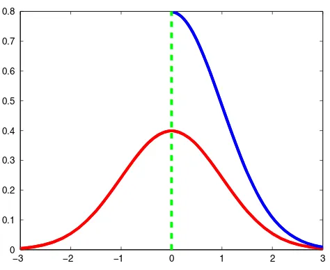
wherel =1, . . . ,d. As shown in Fig.4, the distribution is defined on half domain of a Gaussian distribution but with two times the usual Gaussian amplitude. Therefore, the dis-tribution of|r1|(pit−s
i,n
t )is|r1|(pit−s i,n
t )∼R1, whereR1
is defined on half domain of ad-dimensional Gaussian dis-tribution with a doubled amplitude as follows.
−3 −2 −1 0 1 2 3
0 0.1 0.2 0.3 0.4 0.5 0.6 0.7 0.8
Fig. 4 Pdf for a Gaussian distribution:N(0,1)(red) and for a Gaussian distribution conditioned to have support in[0,+∞): 2N(0,1)(blue)
2N(0,p), p=
⎛ ⎜ ⎜ ⎝
(pit−sit,n)
2 1 0
...
0 (pit −s i,n t ) 2 d ⎞ ⎟ ⎟ ⎠
Similarly,|r2|(gt−sit,n)is distributed on the half domain of the following distributionR2
2N(0,g),g=
⎛ ⎜ ⎜ ⎝
(gt−sit,n)
2 1 0
...
0 (gt −s i,n t ) 2 d ⎞ ⎟ ⎟ ⎠
Together with∼R3=N(0,), the implicit proposal
distribution behind an APSO iteration isR = R1∗R2∗ R32with asit,ntranslation. Here∗stands for the convolution operator.
In this way, the PSO iterations can naturally take the cur-rent observationot into consideration, since{pit}iN=1andgt are updated to their observations. Therefore, with coarse importance sampling from the state transition distribution
p(st|pit−1), the hierarchical sampling process can
approxi-mate to the optimal sampling from p(st|sit−1,ot).
As shown in Fig.5, when the transition distribution is sit-uated in the tail of the observation likelihood, the particles directly drawn from this distribution do not cover a significant region of the likelihood, and thus the importance weights of most particles are low, leading to unfavorable performance. In contrast, through hierarchial sampling process in our algo-rithm, the particles are moved towards the region where the likelihood of observation has larger values, and are finally
2 Since the analytical form ofRis not available, we called it latent
[image:11.595.307.544.77.271.2]Fig. 5 Sampling results after PSO iterations
relocated to the dominant modes of the likelihood, demon-strating the effectiveness of our sampling strategy.
4.3 Differences to Previous Work
Image observations have been utilized for particle guidance in previous workSullivan and Rittscher (2001),Choo and Fleet(2001). In Sullivan and Rittscher (2001), a momen-tum based on the differences between consecutive frames is used to determine the search mechanism and the size of the particle set. Motion prediction based on the differences between consecutive frames is unreliable, especially in the LFR video. Besides, the tracking framework inSullivan and Rittscher(2001) is a particle filter which is not effective in dealing with the abrupt motion in LFR videos. InChoo and Fleet(2001), Choo and Fleet propose a hybrid Monte Carlo technique. Multiple Markov chains are employed to rapidly explore the state space using posterior gradients. The target posterior is approximated by a linear mixture of transition densities and measurement density. However, it is impossi-ble to define a proper transition density, because the object motion is unpredictable in the LFR video, thus leading to an inefficient sampling in the LFR video tracking.
5 Integral Image of Model Parameters
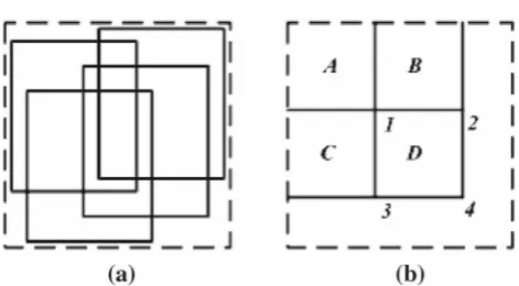
When evaluating the the fitness value of each particle in the APSO iteration process, we need to calculate the parameters of the candidate image region to obtain the similarity measure in Eq. (15). As shown in Fig.6, the candidate image regions corresponding to the particles may have many overlapped areas, and the image pixels inside the overlapping region will be used repeatedly in calculations. This involves large and unnecessary computational load.
5.1 Integral Image Calculation
The motivation is to avoid the unnecessary computation. The idea is to: first, estimate the maximal coverage region of the particle set, and then calculate the label and position features for each pixel. Finally, construct the integral image of these features. The details are described as follows.
Fig. 6 An illustration example
• Estimate the maximal coverage regionof the particle set, that is a region which includes all the possible parti-cles. To determine this set, we require prior information about the object motion. However, in LFR video, it is difficult to estimate the abrupt motion. In our work, we introduce a variableκmaxt which is the absolute value of the maximum velocity in a second up to timet. The max-imal coverage regionfor timet+1 is set to the image area corresponding to [gt −1.2κmaxt ,gt + 1.2κmaxt ], wheregt is the tracking result of the object state at time
t. Here, the maximal coverage region is heuristically selected by utilizing the motion information in the pre-vious tracking process, and thus provides a reasonable bound on the movement of the particles and a certain capability to take account of their acceleration.
• Label each pixel in using the fast assignment algo-rithm in Table 2, and then construct a 5D feature for each pixelqi = {δ(L(i)−l), (pi)x, (pi)y, (pi)x2, (pi)2y}, where δ(L(i)−l)is the Kronecker function such that
δ(L(i)−l)=1 ifL(i)=landδ(L(i)−l)=0 other-wise.(pi)x, (pi)yare, respectively, thexandycoordinate values of the pixeli.
• Construct the integral image of the 5D feature for each color mode. For example, given a position pi, the cor-responding value of the integral image for thelth color mode is
Hil =
pk∈,pk≤pi,L(k)=l
qk
• Calculate the parameters of the candidate image region. Suppose the corresponding image region of a given par-ticle isD, as shown in in Fig.7(b). Similar toViola and Jones(2004), the integral image of this region for thelth color mode can be easily obtained by four table lookup operations H4l+H1l −H2l −H3l. As a result, the para-meters of this particle can be obtained from Eqs. (8), (9) and (10).
[image:12.595.56.305.82.160.2] [image:12.595.300.542.82.191.2]Fig. 7 aSolid line: Particle set,dashed line: the coverage region.bAn illustration of calculation therectangleintegral image
Wang et al.(2007), the particle filtering framework is used and thus it is easy to obtain the coverage regionof par-ticle set after the parpar-ticle generation process. The parpar-ticles change in the iterations of particle swarm optimization and thus it is more difficult to estimate the coverage region of all possible particles. (2) Pixels insideare labeled by a nearest neighbor classifier inWang et al.(2007). In our work, labelling is realized by the dominant-set fast assign-ment algorithm.
5.2 Computational Complexity Analysis
In summary, the features of each pixel need to be calcu-lated only once even though the APSO algorithm is iterative. The complexity is analyzed as follows: In the APSO based searching process, there are two parameters which affect the computational complexity: the number of particlesNand the iteration number M. Let Y be the computational complex-ity for evaluating one particle without the integral image, let
ybe the computational complexity for evaluating one parti-cle with the integral image, and letC be the computational complexity for building the integral image. The total com-putational complexity without the integral image isN MY. While with the integral image built in this section, the compu-tational complexity isN M y+C. In more detail,yincludes the cost of a set of table lookup operations and the direct computation in Eq. (15), and satisfiesyY. The value ofC
depends on the experimental data, and we haveC/Y <10 in our experiments. AssumingC/Y =10 and ignoring y, the integral image strategy can achieve N M yN MY+C = N M10 times speed up. The relationships amongY,y,C are validated in our experiments.
6 Experimental Results
In this section, we first carry out two experiments with syn-thetic data to analyze and validate the claimed advantages of the bin-ratio based distance measure and the annealed
par-ticle swarm optimization based searching method. Then we test the proposed tracking system in the following aspects on real data: different object representations, different similarity measures, different searching methods, different frame rates and average running time. All the experiments are conducted with Matlab on a platform with Pentium IV 3.2GHz CPU and 512M memory. The initial object positions are manually labeled.
6.1 Synthetic Analysis of Bin-Ratio Based Distance Measure
To validate the claimed advantages of the bin-ratio based distance measure, we compare it with the histogram inter-section measure (Swain and Ballard 1991) in the presence of illumination changes and image clutters.
6.1.1 Robustness to Illumination Changes
In this part, we assume that the target region is represented by a 20×20 patch in which the pixel values are drawn from a uniform distribution over{0,1, . . . ,255}. The cor-responding histogramu1is obtained by uniformly grouping
the pixels into 16 bins.3When the illumination changes, we assume that the intensities of a ratioς∈ [0,100 %]of pixels within the patch change by a factormin the range[1/5,5] (the intensities of pixels are set to 255 if their values are bigger than 255 after illumination changes), and the cor-responding histogram isu2. For comparison, we generate
another histogramu3in a similar way tou1, for reference.
For the bin-ratio based distance, since it is a distance mea-sure,c(u1,u2) < c(u1,u3)indicates the robustness to
illumination changes. While the histogram intersection dis-tanceQ(·,·)is a similarity measure,Q(u1,u2) >Q(u1,u3)
shows its robustness to illumination changes. We repeat this process for 10,000 times and calculate the frequency that these inequalities are correct for variousmandς. The exper-imental results are reported in Table3.
The results in Table3are analyzed in two aspects as fol-lows.
1. Let us first focus onς. Both measures have poor per-formance when ς > 50 %. The reason is that: when the intensities of more than 50 % pixels increase or decrease by the same factor (simulating for the illumi-nation changes), and then these pixel values shift to the bins of hight intensity value or low intensity value. As a result, the corresponding histogramu2 is very different
from the uniform histogramu1. In addition,u1andu3are
both generated in the same way, and they are all nearly
3 Since the patch is generated by a uniform distribution, the dominant
Table 3 The accuracies of different measures with different
values ofςandm
ς Method m=15 m=14 m=13 m= 12 m=2 m=3 m=4 m=5
ς=10 % c(·,·) 0.982 0.988 0.987 0.984 0.983 0.983 0.977 0.968
Q(·,·) 0.996 0.999 0.999 0.999 0.998 0.994 0.99 0.983
ς=20 % c(·,·) 0.844 0.887 0.956 0.967 0.88 0.758 0.633 0.508
Q(·,·) 0.675 0.801 0.898 0.957 0.817 0.547 0.353 0.256
ς=30 % c(·,·) 0.337 0.457 0.656 0.817 0.549 0.202 0.106 0.062
Q(·,·) 0.081 0.15 0.402 0.728 0.318 0.05 0.017 0.005
ς=40 % c(·,·) 0.034 0.07 0.207 0.504 0.181 0.025 0.007 0.002
Q(·,·) 0.002 0.008 0.05 0.334 0.06 0 0 0
ς=50 % c(·,·) 0.001 0.005 0.022 0.155 0.034 0.001 0 0
Q(·,·) 0 0 0.002 0.089 0.007 0 0 0
ς=60 % c(·,·) 0 0 0 0.023 0.003 0 0 0
Q(·,·) 0 0 0 0.016 0 0 0 0
ς=70 % c(·,·) 0 0 0 0 0 0 0 0
Q(·,·) 0 0 0 0 0 0 0 0
ς=80 % c(·,·) 0 0 0 0 0 0 0 0
Q(·,·) 0 0 0 0 0 0 0 0
ς=90 % c(·,·) 0 0 0 0 0 0 0 0
Q(·,·) 0 0 0 0 0 0 0 0
Better performance values are given in bold
uniform distributions. Therefore, finding a correct match amongu1,u2andu3 is really a challenging task. Ifu3
is generated from a Gaussian distributed patch, then the performance of two measures will significantly improve andc(·,·)still outperformsQ(·,·)in most cases. 2. c(·,·)performs better thanQ(·,·)in most cases except
ς =10 %. In this case, only 10 % of pixels are affected by illumination changes, and the bins of the histogram are influenced only slightly after normalization. There-fore the histogram intersection distance Q(·,·)changes only slightly. However, whenς >20 %, more pixels are contaminated which cause the imbalance between differ-ent bins and the bin-ratios can deal the imbalance more better.
6.1.2 Robustness to Image Clutter
In this part, we assume the target is randomly corrupted by image clutter, e.g. background noise and partial occlusion. As before, u1 represents the histogram of the target. The
image clutter is simulated as follows. We randomly select a ratioς ∈ [0,100 %]pixels within the patch and replace the intensity values of these pixels by a certain valuem∗255. The resulting histogramu2represents the target under image
clutter.
The parameters in this experiment are set as follows:
ς ∈ [0,100 %]is the proportion of bins influenced by the image clutter, and m is sampled uniformly from[0,1]. In this experiment,u3is generated from a Gaussian distributed
patch with mean 128 and standard deviation 32.4The exper-iment is run for 10,000 times, and the proportion of distance comparisons that correctly matchu1andu2is recorded. The
experimental results are reported in Table4.
The results in Table 4 are analyzed as follows. First,
c(·,·)outperformsQ(·,·)in all cases. This shows that the bin-ratio used for evaluation is more robust to the image clut-ter. Second, we find that bothc(·,·)andQ(·,·)have a poor performance whenς >50 %. This reasonable because more than 50 % pixels are background or occluded which causes incorrect matching.
6.2 Synthetic Analysis of Annealed Particle Swarm Optimization
In this part, APSO is tested on a popular non-linear state estimation problem, which is described as a benchmark in many papers (Merwe et al. 2000). Consider the following nonlinear state transition model given by
st =1+sin(π(t−1))+φ1st−1+γt−1, st ∈R (29)
whereγt−1is a GammaGa(3,2)random variable modeling
the process noise, and =4e−2 andφ1=0.5 are scalar
parameters. A non-stationary observation model is as follows
4 Pixels are replaced to simulate image clutter which is more
challeng-ing than scalchalleng-ing by a factor in case of illumination changes. For this reason the entries ofu3are not uniform in size. For more detail, please
Table 4 The accuracies of different measures with different
values ofςandm
ς Method m=0 m= 17 m=27 m=73 m= 47 m=57 m=67 m=1
ς=10 % c(·,·) 1 1 1 1 1 1 1 1
Q(·,·) 1 1 1 1 1 1 1 1
ς=20 % c(·,·) 1 1 1 1 1 1 1 1
Q(·,·) 1 1 1 1 1 1 1 1
ς=30 % c(·,·) 1 1 1 1 1 1 1 1
Q(·,·) 0.936 0.941 0.946 0.924 0.937 0.945 0.928 0.941
ς=40 % c(·,·) 0.999 0.999 1 1 1 1 1 1
Q(·,·) 0.003 0.001 0.005 0 0.001 0.003 0.002 0.001
ς=50 % c(·,·) 0.387 0.387 0.372 0.372 0.381 0.358 0.398 0.326
Q(·,·) 0 0 0 0 0 0 0 0
ς=60 % c(·,·) 0.001 0.001 0.001 0 0 0 0 0
Q(·,·) 0 0 0 0 0 0 0 0
ς=70 % c(·,·) 0 0 0 0 0 0 0 0
Q(·,·) 0 0 0 0 0 0 0 0
ς=80 % c(·,·) 0 0 0 0 0 0 0 0
Q(·,·) 0 0 0 0 0 0 0 0
ς=90 % c(·,·) 0 0 0 0 0 0 0 0
Q(·,·) 0 0 0 0 0 0 0 0
ot =
φ2xt2+nt, t ≤30
φ3xt−2+nt, t >30 (30)
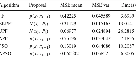
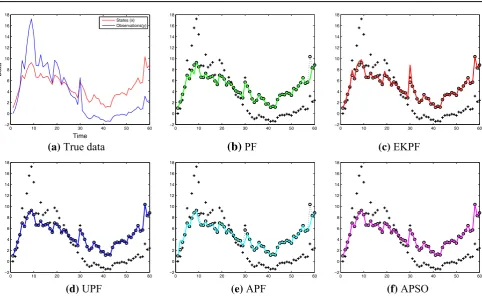
whereφ2 =0.2, φ3 =0.5, and the observation noisent is drawn from a Gaussian distributionN(0,0.00001). Given only the noisy observation ot, several filters are used to estimate the underlying state sequencest fort = 1. . .60. Here, we compare APSO with conventional particle filter (Arulampalam et al. 2002), extended Kalman based particle filter (Freitas et al. 2000), unscented particle filter (Merwe et al. 2000), auxiliary particle filter (Pitt and Shephard 1999), and conventional particle swarm optimizationKennedy and Eberhart (1995).5 For each algorithm, a proposal distrib-ution is chosen as shown in Table 5. The parameters in
APSO and PSO are set as follows: = 0.8,c = 2,
ϕ1 = ϕ2 = 1, ξmax = 0.8, ξmi n = 0.1,T = 20. Figure
8gives an illustration of the estimates generated from a sin-gle run of the different filters. Compared with other nonlinear filters, APSO is more robust to the outliers, when the observa-tion is severely contaminated by the noise. Since the result of a single run is a random variable, the experiment is repeated 100 times with re-initialization to generate statistical aver-ages. Table5summarizes the performance of all the different filters in the following aspects: the means, variances of the mean-square-error (MSE) of the state estimates and the aver-age execution time for one run. It is obvious that the averaver-age accuracy of APSO is better than generic PF, EKPF, APF and
5We call these filters APSO, PF, EKPF, UPF, APF, PSO respectively
for short in the following parts.
Table 5 Experimental results of state estimation
Algorithm Proposal MSE mean MSE var Time(s)
PF p(xt|xt−1) 0.42225 0.045589 3.6939
EKPF N(x¯t,P¯t) 0.31129 0.015167 13.014
UPF N(x¯t,P¯t) 0.06977 0.024894 26.2815
APF p(xt|xt−1) 0.55196 0.037047 7.1835
PSO p(xt|xt−1) 0.13019 0.044086 10.2087
APSO p(xt|xt−1) 0.060502 0.06852 6.8005
comparable to that of UPF. However, the real-time perfor-mance of our algorithm is much better than UPF as Table
5shows. Meanwhile, we can see that APSO can achieve a much faster convergence rate than conventional PSO. This is because the velocity part employed in Eq. (19) carries lit-tle information, while the annealing part in APSO iterations enhances the diversity of the particle set and its adaptive effect enables a fast convergence rate. In summary, the total performance of APSO prevails over that of other nonlinear filters.
In order to further evaluate the sampling effectiveness of the hierarchical sampling process in APSO, we consider a special case of the state space model as follows:
st = f(st−1)+γt−1, γt−1∼N(0,10) (31)
ot =
st
20+nt, nt ∼N(0,1) (32)
where f(st−1)= st2−1+125+sst2−1
t−1+
[image:15.595.308.544.380.481.2]