An Empirical Investigation of the Monetary Model Economic Fundamentals

(1)

http://www.scirp.org/journal/me ISSN Online: 2152-7261

ISSN Print: 2152-7245

An Empirical Investigation of the Monetary Model

Economic Fundamentals

Jean René Cupidon

1

, Judex Hyppolite

2

1_{Department of Economics and Mathematics, Berea College, Berea, KY, USA}

2_{Department of Economics, Finance, and Real Estate, Monmouth University, West Long Branch, NJ, USA}

Abstract

This paper presents an empirical investigation of an important series called “eco-nomic fundamentals” derived from the flexible price monetary model of exchange rate determination. The model predicts that the nominal exchange rate is determined by the “economic fundamentals”, referred here as the series ft. As a result, the cha-racteristics of the “economic fundamentals” process may influence the properties of the nominal exchange rate process. We will just use the term “fundamentals”. Nev-ertheless, many exchange rate models found in the literature assume an ad-hoc process for ft ignoring the fact that the specification of this process can be formally derived within the framework of the monetary model. Using data for several coun-tries on GDP and money supplies, we construct the series ft according to the mon-etary model specification, and we examine some important characteristics of its empirical distribution such as skewness, kurtosis, stationarity, ARCH and GARCH properties. We observe that the series is not exactly normally distributed, as com-monly assumed in many target zone models. This investigation essentially helps with modeling exchange rate and more importantly in the analysis of exchange rate target zones modeling by identifying potential restrictions that need to be taken into con-sideration when choosing a process for the modeling of the “economic fundamen-tals”.

Keywords

Exchange Rates, Time Series

1. Introduction

The monetary model was originally developed as a framework to analyze Balance-of- payments adjustments under a fixed exchange rate regime and has been modified after

How to cite this paper: Cupidon, J.R. and Hyppolite, J. (2016) An Empirical Investiga-tion of the Monetary Model Economic Fun- damentals. Modern Economy, 7, 1728-1740.

http://dx.doi.org/10.4236/me.2016.714151

Received: November 10, 2016 Accepted: December 18, 2016 Published: December 21, 2016

http://creativecommons.org/licenses/by/4.0/

(2)

the Breakdown of the Bretton Woods system as a model of nominal exchange rate de-termination. The model is a common theme in textbooks on open-economy macroe-conomics and in the literature. In addition, the model forms the basis of most target zone models and balance-of-payments studies. However, several versions of the mone-tary model have been developed over the years. In fact, Dornbusch [1] developed a sticky-price version of the model while Frenkel [2] and Mussa [3] developed a flexible price version. Dornbusch’s sticky-price monetary model allows for short-run over-shooting of the nominal exchange rate above its long-run value that is associated with purchasing power parity (PPP). But, according to Frankel (1979), the Sticky-price monetary model contains a deficiency in that it does not explicitly incorporate short- run difference in secular rates of inflation between the two countries. To overcome this shortcoming, he introduced the real interest differential monetary model that combines elements of both the flexible-price and sticky-price monetary models.

1.1. Derivation of the Exchange Rate Process

The symbol  is used to denote foreign variables. A building block of the monetary model is purchasing power parity (PPP). The model makes four basic assumptions: 1) Money market equilibrium;

2) Continuous stock equilibrium in the money market; 3) Uncovered interest parity (UIP); and

4) Purchasing power parity.

Monetary equilibrium conditions in the domestic and foreign markets are given re-spectively by

t t t t

m −p =φy −αi (1)

v

t t t t

m−p =φ y −α i

(2) The parameter φ is known as the income elasticity of money demand where

0< <φ 1 and α is the interest rate semi-elasticity of money demand.

International capital market equilibrium is given by assuming that uncovered inter-est parity holds, that is,

1 , t t t t t

i −i =s₊ −s (3) where _t

( )

. denotes expectation operator conditional on all publicly available

infor-mation to economic agents at time t. Also, PPP states that st =pt−pt

_{. PPP is assumed}

to hold continuously in the model. Empirical studies show that PPP is violated in the short run but may hold in the long run. Now, we obtain

(

) (

=

) (

)

t t t t t t t t

m −m− p −p

φ

y −

φ

 y −

α

i −

α

 i

(4)

Using the PPP condition, we obtain the fundamental equation of the flexible price monetary model

(

) (

)

t t t t t t t

(3)

As commonly done in the literature, we simplify the model by assuming that the in-come elasticities and interest rate semi-elasticities of money demand are the same for the domestic and foreign countries. In this case, the fundamental equation becomes

(

) (

)

t t t t t t t

s =m −m −

φ

y −y +

α

i −i

(6)

At this point, we can use the UIP condition to obtain

(

)

(

1

)

,

t t t t t t t

s =m −m−

φ

y −y +

α

 ∆s₊

(7)

Following Nelson Mark, we let

(

)

t t t t t

f =m −m−

φ

y −y (8)

We therefore obtain

(

1

)

,

t t t t

s = f +α ∆s₊ (9) This last version constitutes the fundamental equation of the flexible price monetary model in discrete time. This equation is basically a first order stochastic difference equ-ation in the variable st in expectation form.

The expression for ft is referred to as the “economic fundamentals” or the funda-mental determinants of exchange rate determination.

To solve for st, it is more useful to rewrite the equation as follows 1

t t t t

s =γ f +ψs+

(10)

where 1

1

γ

α

=

+ and 1

α

ψ

α

=

+ . This class of stochastic difference equations is usually solved by the method of undetermined coefficients or by repeated substitutions. This equation states that expectations of future values of the exchange rate, that is, t ts+1,

are embodied in the current exchange rate. It also indicates that high relative money growth in the domestic country leads to a weakening of the home currency, while an increase in the relative domestic income leads to a strenghtening of the home currency. We can write

1 1 1 2

t t t t

s+ =γ f+ +ψ+s+

(11)

It follows that

1 1 1 2

1 2

t t t t t t

t t t t

s f s

f s γ ψ γ ψ + + + + + + = + = +   

 

(12)

It follows that

2

1 1 1

2

1 2

t t t t t t t t

t t t t t t

s f f s f

f f s

γ ψ ψγ

γ γψ ψ

+ + +

+ +

= + + +

= + +

  

(13)

In a similar fashion we obtain

2

1 3

t t t t t t t

s =γ f +γψ f₊ +γψ s₊ (14) Continuing the process, we obtain the following recursive equation

1 1 0

k

j k

t t t j t t k

j

s γ ψ f₊ ψ + s_{+ +} =

(4)

If the following transversality condition

lim k 0,

t t k

k→+∞ψ s+ =

(16) is imposed, we obtain the so-called “no-bubbles” or “rational expectations” solution by letting k go to infinity:

0 j

t t t j

j s γ ψ f

∞

+ =

=

∑

_

₍₁₇₎

The transversality condition puts a constraint on the rate at which the exchange rate can grow.

The “no-bubbles” solutions indicates that the exchange rate is the present value of expected future values of the economic fundamentals. This is in view with the “asset” approach to the exchange rate according to which the exchange rate should be expected to behave just like other assets, such as stocks and bonds.

1.2. Interactions between the Properties of the Fundamental Process

and Those of the Exchange Rate Process

We see that the exchange rate is a function of the fundamentals process. Therefore, the properties of the fundamentals have serious implications on the properties of the ex-change rate process. Conversely, the observed characteristics of the exex-change rate series put some restrictions on the potential characteristics of the fundamentals process. In this section we look at the implications of some well known stylized facts about ex-change rate data for the characteristics of the fundamentals series.

For empirical purposes, we follow Mark characterization setting ψ =1 and use the

expression

(

)

t t t t t

f =m −m− y −y (18)

Two common stylized facts are as follows:

1) The deviation of the price from the fundamentals displays substantial persistence and much less volatility than the exchange rate returns.

2) The volatility of exchange rate returns, that is of ∆st, is virtually indistinguishable from stock return volatility.

At this stage of the analysis, we want to focus on some empirical analysis by specifi-cally looking at some descriptive statistics about the economic fundamentals, ft, as de-fined in (0.18).

To address the excess volatility in the exchange rate returns relative to changes in the fundamentals, as in Mark [4], the growth rate of the economic fundamentals is as-sumed to follow the following AR(1) stationary process

1

t t t

f ρ f−

∆ = ∆ + (19) where t is assumed iid with mean 0 and variance

2

σ_. No normality assumption is necessary.

The k-step ahead prediction formula is

(

)

j

t ∆ft+j =

ρ

∆ft

(5)

Alternatively, we obtain

( )

1 1 1 1 1 1 j j

t t j t t

k j

t t

j

t t t

f f f

f f

f f f

ρ ρ ρ ρ ρ ρ ρ ρ ρ + = = + ∆ − = + ∆ − = + ∆ − ∆ − −

∑



We then obtain

( )

(

)(

)

(

)(

)

0

0 0 0

1

1 1

1 1 1 1 1

j j

t t t t

j

j j

j

t t t

j j j

t t t

s f f f

f f f

ρ

γ ψ ρ ρ

ρ ρ

ψρ ψ

γ ψ γ ρ γ ρ

ρ ρ

γ γρ γρ

ψ ψ ρ ρψ ρ

∞ = ∞ ∞ ∞ = = =   = _ + ∆ − ∆ _ − −   = + ∆ − ∆ − − = + ∆ − ∆ − − − − −

∑

Thus, the exchange rate solution can be simplified and we have the following formula

(

)

(

)(

)

1 1

1 1 1

1

1 1 1

1 1

t t t

t t

s f f

f f

ργ

ρ ψ ρψ

ψ ρ

ργ

ρ ψ ρψ

γ _ψ ρ

ψ ρψ   = + _ − _∆ − _ − − _  −  = + _ _∆ − _ − − _     = +_ _{ } _∆ − −    

Thus, we obtain the exchange rate solution to the standard FPMM

1

t t t

s f ρψ f

ρψ

 

= +_ _∆

−

  (21)

At this point, we want to compare the variance of the exchange rate returns, ∆st with the variance of the change in fundamentals, ∆ft. We have

( )

(

)

( )

(

)

(

)

1 1

1

1 2 1

2 2

1 2 1 1 2 1

1 1

1

1 1

2 ,

t t t t t

t t

t t t t

ar s ar f f f f

ar f f

ar a f a f

a ar f a ar f a a ov f f

ρψ ρψ ρψ ρψ ρψ ρψ ρψ − − − − − −       ∆ = _ +_ _∆ − −_ _∆ _ − −         = _ ∆ − ∆ _ − −   = ∆ + ∆ = ∆ + ∆ + ∆ ∆       

Since the series

{ }

∆ft is assumed to be stationary, then we have

( )

t

(

t 1

)

ar ∆f = ar ∆f₋

  and ov

(

∆ ∆ft, ft−1

)

=ρar

( )

∆ft . Therefore, we obtain

( )

(

)

(

( )

)

(

)

( )

(

)

(

)

(

)

( )

2 2 2

2

2 2 2 2 2 2 1 2 1 1 2 1

1 2 1

1

t t t t

t

ar s ar f ar f ar f

ar f

ρ ψ ρ ψ

ρψ

ρ ψ ρ ψ

ρψ

ρψ ρψ ρ

(6)

Hence, we see clearly that

( )

_t

( )

.

t ar ∆s > ar ∆f

[image:6.595.194.552.408.686.2]

  (22)

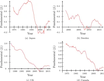
Figure 1 shows that the series in level

{ }

ft are not stationary. If they have unit root

the AR(1) process specified above for the economic fundamentals does not explain the empirical fact that exchange rate returns are more volatile than the growth rate of the fundamentals.

2. Some Characteristics of the Empirical Distribution of the

Fundamentals

Given the implications of the properties of the fundamentals for the characteristics of the exchange rate process, it is important to analyze some essential aspects of the em-pirical distribution of the fundamentals,

{ }

ft .

2.1. Some Sample Statistics

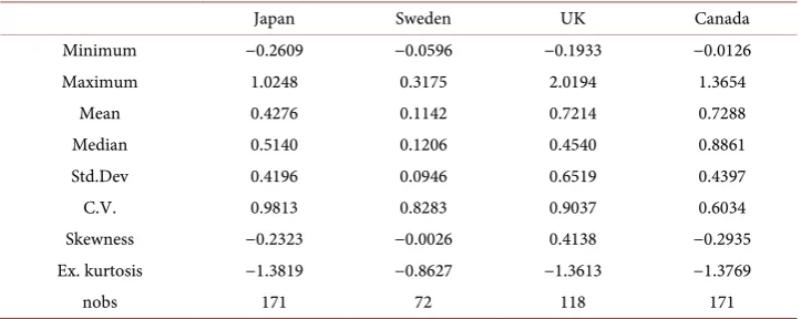
First, we present a set of sample statistics in Table 1. The series

{ }

ft is computed

us-ing quarterly data on money supplies on both the domestic and foreign countireis from

3 1

1973Q −2016Q for Japan and Canada, from 1998Q2−2016Q1 for Sweden, and from

1 1

1987Q −2016Q for the United Kingdom. Quarterly GDP is usually unavailable for most countries. Therefore, an Industrial production index is usually used as a proxy for national income. The data are available on the website of the OECD. One important goal is to assess the similarity of the distribution of the series

{ }

ft to the normal dis-

(7)

[image:7.595.193.555.105.249.2]

Table 1. Descriptive statistics on the economic fundamentals

( )

{ }

ft for Japan, Sweden, UK, and

Canada.

Japan Sweden UK Canada

Minimum −0.2609 −0.0596 −0.1933 −0.0126

Maximum 1.0248 0.3175 2.0194 1.3654

Mean 0.4276 0.1142 0.7214 0.7288

Median 0.5140 0.1206 0.4540 0.8861

Std.Dev 0.4196 0.0946 0.6519 0.4397

C.V. 0.9813 0.8283 0.9037 0.6034

Skewness −0.2323 −0.0026 0.4138 −0.2935

Ex. kurtosis −1.3819 −0.8627 −1.3613 −1.3769

nobs 171 72 118 171

tribution. As a result, we will first look into the sample or empirical coefficient of kur-tosis commonly defined as

(

)

(

)

4 1

2 2 1

1

. 1

T t t

Y Y

T

Y Y T

κ

=

= − =

 ₋ 

 

 

∑

It is clear that the distribution of the

{ }

ft series is not normal as indicated at least

by the excess kurtosis. Since the skewness is negative for Sweden and Japan, the data skewed to the left, that the left tail is longer. But, given that the skewness is between −0.5 and 0.5, the distribution can be viewed as approximately symmetric. Figure 2

shows the density of the economic fundamentals estimated using a normal kernel. A quick observation confirms our analysis, particularly for Japan and Sweden. From this analysis, we observe that the series

{ }

ft does not appear to have a

nor-mal distribution.

Let S f

( )

be the coefficient of skewness and κ

( )

f be the coefficient of kurtosis. We can also test the hypotheses:

1) H0:S f

( )

=0; Ha:S f

( )

≠0

2) H0:κ

( )

f − =3 0; Ha:κ

( )

f − ≠3 0

The t-statistics for the above tests as well as the corresponding p-value are presented in Table 2. Additionally, the Jarque and Bera [5] statistics, which can be viewed as a combination of the above statistics is also presented.

According to the table at a 5% significance level we cannot reject the hypothesis that the distributions of the series are symmetric, but we can reject the hypothesis of zero excess kurtosis as well as the hypothesis of normality.

This analysis may seem unnecessary. However, it actually has very important impli-cations in terms of exchange rate modeling in both the discrete and continuous time as well as aset pricing modeling. The following section tackles the issue of stationarity.

2.2. Stationarity of the Fundamentals

(8)

[image:8.595.234.553.64.370.2]

Figure 2. Density estimation.

Table 2. Test of normality.

skew tskew p-value kurt tkurt p-value JB p-value

Japan −0.2323 −1.2403 0.2149 1.6181 4.3191 0.0000 20.1927 0.0000

Sweden −0.0026 −0.0089 0.9929 2.1373 3.7019 0.0002 13.7039 0.0011

UK 0.4138 1.8349 0.0665 1.6387 3.6336 0.0003 16.5696 0.0003

Canada −0.2935 −1.5669 0.1171 1.6231 4.3325 0.0000 21.2260 0.0000

the series is stationary or non stationary. The examination of stationarity is important because doing regression analysis with non stationary time series can lead to spurious regression results. We now tackle this question for each of the

{ }

ft series considered

above, namely for respectively US-JAPAN series, US-SWEDEN, US-CANADA, and US-UK data on output and money supplies from 1973 :Q1 to 1997 :Q4 (Figure 3 &

Figure 4).

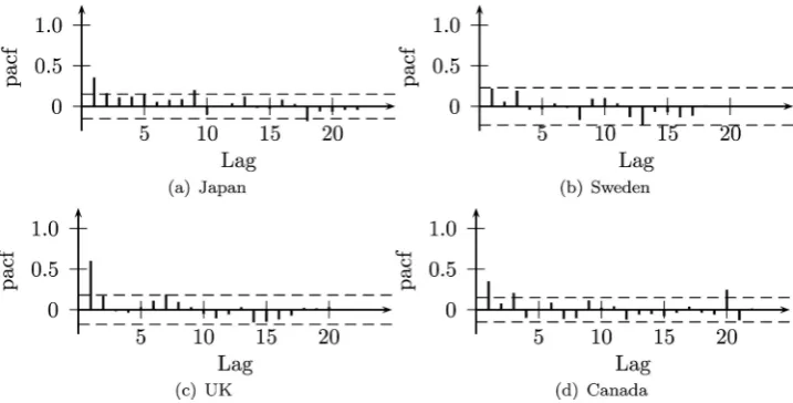
[image:8.595.40.555.414.498.2]

(9)

Information criterion is an AR(9) and since the autocorrelation coefficients are signifi-cant for several lags, the autoregressive model of order 9 appears to be a good model for this series. A similar analysis for Sweden, the United Kingdom, and Canada suggest that we work with autoregressive processes of order 1, 2, and 3 respectively.

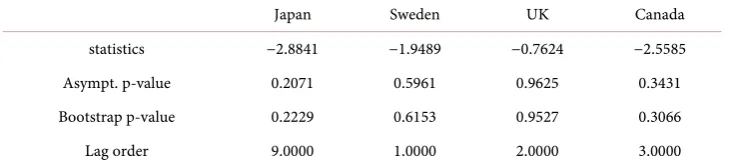
[image:9.595.195.555.277.455.2]

The Augmented Dickey Fuller test that follows is based on the above autoregressive models. The test’s null hypothesis assumes that the series is non stationary while the al-ternative hypothesis states that the series is stationary. Since the distribution of the ADF test statistic under the null hypothesis is not the usual t-distribution, Monte Carlo me-thods are used approximate the distribution of the statistic. The null hypothesis of non-stationarity is rejected as long as the test statistic is smaller than a commonly specified critical value or the associated p-value is less than a chosen significance level. Other-wise, stationarity should be maintained. In Table 3 the p-value are computed using Monte Carlo methods and model-based bootstrap. The latter is chosen to account for

Figure 3. Sample autocorrelation function of the quaterly change in the fundamentals for Japan,

Sweden, the United Kingdom, and Canada.

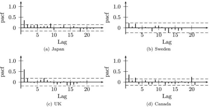
Figure 4. Sample partial autocorrelation function of the quarterly change in the fundamentals for

[image:9.595.195.554.495.677.2]

(10)

[image:10.595.192.557.91.175.2]

Table 3. Augmented dickey fuller test.

Japan Sweden UK Canada

statistics −2.8841 −1.9489 −0.7624 −2.5585

Asympt. p-value 0.2071 0.5961 0.9625 0.3431

Bootstrap p-value 0.2229 0.6153 0.9527 0.3066

[image:10.595.194.554.206.274.2]

Lag order 9.0000 1.0000 2.0000 3.0000

Table 4. KPSS test.

Japan Sweden UK CANADA

statistics 2.6537 1.8265 3.6722 4.2132

p-value 0.0100 0.0100 0.0100 0.0100

Lag order 3.0000 1.0000 2.0000 3.0000

the low power of ADF test reported in the literature.

The KPSS test procedure is more commonly used in empirical work. The null hypo-thesis is that the series is stationary. Here, for completeness, we report both testing procedures.

Table 3 shows that for all the series the Asymptotic and the Bootstrap p-values are greater than 20%. We cannot reject the null hypothesis that the series are non-stationary. This observation is confirmed in Table 4 where the p-values of the KPSS test are all less than or equal to 1%, which provides evidence against stationarity.

To complete the analysis, we explore whether the series exhibit Autoregressive Con-ditional Heteroskedasticity (ARCH) or Generalized ARCH (GARCH) effects. Stock prices usually exhibit ARCH and GARCH properties. Moreover, given that most inter-national economists believe that exchange rates behave like stock prices, we would ex-pect exchange rates to have such properties. We will examine ARCH and GARCH ef-fects in the next section.

2.3. ARCH and GARCH Effects for the Fundamentals

We examine the conditional variance of the above four series to determine the presence of ARCH and GARCH effects. We start by estimating the conditional means of the se-ries by determining the ARMA model that minimizes the Akaike Information criterion. We then generate the residuals which are used to compute the sample autocorrelation function and the sample partial autocorrelation functions of the squared residuals. They are plotted in the following figures (Figure 5 & Figure 6).

According to the sample autocorrelation functions of the square of the residuals, Ja-pan and the UK cannot be modeled as a pure Moving Average process. However, a Moving Average process of order 0 seems to be appropriate for Sweden, and in the case of Canada one may be able to use a Moving Average process of order 3.

(11)

[image:11.595.197.551.67.248.2]

Figure 5. Sample autocorrelation function of the square of the residuals obtained from the auto-regressive model that minimizes the Akaike Information criterion (AIC).

Figure 6. Sample partial correlation function of the square of the residuals obtained from the

autoregressive model that minimizes the Akaike Information criterion (AIC).

del; for the UK an AR(1) model may be appropriate; the series for Sweden seem to be white noise, while for Canada the partial autocorrelation function seems to point to-ward an AR(3). The above observation suggests an ARCH(1) for Japan, an ARCH(1) for the UK, a GARCH(3,3) for Canada, and no ARCH effect for Sweden.

We also use the Akaike information criterion (AIC) to identify the best autoregres-sive models for the square of the residuals. The models obtained are ARCH(1) for Japan and the UK and ARCH(0) for Sweden and Canada.

[image:11.595.196.553.289.472.2]

(12)

(AR(9)) and then run the regression

2 2 2

0 1 1 2 2

ˆ_t ˆ_t ˆ_t _t

e =γ +γe₋ +γ e₋ +v (23) Of course, vt is an error term. The null hypothesis is H0:γ1=0,γ2 =0 versus 1:at least one coefficient is not 0

H . The null hypothesis states that there are no ARCH

effects. More generally, for the general case, the null hypothesis states that all the coeffi-cients should be zero and the alternative hypothesis states that at least one coefficient should be zero. The LM statistic is

(

)

2

LM = T−q R , where T is the sample size an q is the number of lags _ˆ2

t

e (here q = 1) and R2 is the coefficient of determination. Under the null hypothesis, the LM statistic has a chi-square distribution with q degrees of freedom in large samples. Hence, the null hypothesis is rejected if

(

)

2 2

1 ,q T−q R >

χ

−_α or the associated p-value is less than the chosen significance level, and conclude that ARCH effects are present in the data. The test was implemented and the results are provided in Table 5.

As the table indicated there is evidence in favor of conditional heteroskedasticity for Japan and the UK, but we cannot reject the hypothesis that residuals for Sweden and Canada are white noise.

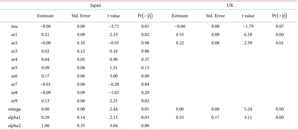
[image:12.595.193.551.380.452.2]

The estimates of the corresponding ARCH models for Japan and the UK are pre-sented in Table 6.

Table 5. LM test for ARCH effect.

LM statistic p value ARCH order (q)

Japan 26.90 0.00 2.00

Sweden 0.97 0.33 1.00

UK 22.25 0.00 2.00

Canada 1.82 0.18 1.00

Table 6. Estimates of the parameters AR-ARCH models for Japan and the UK.

Japan UK

Estimate Std. Error t value Pr

( )

>t Estimate Std. Error t value Pr

( )

>t

mu −0.00 0.00 −2.71 0.01 −0.00 0.00 −1.79 0.07

ar1 0.21 0.09 2.33 0.02 0.55 0.09 6.18 0.00

ar2 −0.00 0.10 −0.03 0.98 0.22 0.08 2.59 0.01

ar3 0.02 0.12 0.18 0.86

ar4 0.04 0.05 0.90 0.37

ar5 0.09 0.06 1.51 0.13

ar6 0.17 0.06 3.00 0.00

ar7 −0.01 0.06 −0.20 0.84

ar8 −0.09 0.09 −1.05 0.29

ar9 0.13 0.06 2.25 0.02

omega 0.00 0.00 2.44 0.01 0.00 0.00 5.24 0.00

alpha1 0.29 0.14 2.13 0.03 0.53 0.17 3.11 0.00

[image:12.595.42.554.480.703.2]

(13)

3. Conclusion

In this paper, we have analyzed some empirical aspects of the economic fundamentals that is shown to be the driving force of exchange rate behavior. The analysis shows that this fundamental series does not appear to be normally distributed as indicated by the excess kurtosis and skewness as well as the estimated kernel density as indicated by the data for several countries. Also, we observe that some ARCH effects are present for most data while GARCH effects are not that common. This has important implications for modeling exchange rate and also the analysis of target zone models.

References

[1] Dornbusch, R. (1976) Expectations and Exchange Rate Dynamics. Journal of Political Eco- nomy, 84, 1161-1176. https://doi.org/10.1086/260506

[2] Frenkel, J.A. (1976) A Monetary Approach to the Exchange Rate: Doctrinal Aspects and Empirical Evidence. Scandinavian Journal of Economics, 78, 200-224.

https://doi.org/10.2307/3439924

[3] Mussa, M. (1976) The Exchange Rate, the Balance of Payments, and Monetary and Fiscal Policy under a Regime of Controlled Floating. Scandinavian Journal of Economics, 78, 229- 248. https://doi.org/10.2307/3439926

[4] Mark, N.C. (2001) International Macroeconomics and Finance: Theory and Econometric Methods. Wiley-Blackwell.

[5] Jarque, C.M. and Bera, A.K. (1987) A Test for Normality of Observations and Regression Residuals. International Statistical Review, 55, 163-172. https://doi.org/10.2307/1403192

Submit or recommend next manuscript to SCIRP and we will provide best service for you:

Accepting pre-submission inquiries through Email, Facebook, LinkedIn, Twitter, etc. A wide selection of journals (inclusive of 9 subjects, more than 200 journals)

Providing 24-hour high-quality service User-friendly online submission system Fair and swift peer-review system

Efficient typesetting and proofreading procedure

Display of the result of downloads and visits, as well as the number of cited articles Maximum dissemination of your research work