Munich Personal RePEc Archive
Technological progress and economic
growth: evidence from Poland
Gurgul, Henryk and Lach, Łukasz
2012
Online at
https://mpra.ub.uni-muenchen.de/52279/
1
Technological progress and economic growth:
Evidence from Poland
Henryk Gurgula,*, Łukasz Lachb
a
Department of Applications of Mathematics in Economics, Faculty of Management, AGH University of Science and Technology, Gramatyka 10 st., 30–067 Cracow, Poland, tel.: +48 012 6174310, fax: +48 012 6367005, e–mail: henryk.gurgul@gmail.com.
b
Department of Applications of Mathematics in Economics, Faculty of Management, AGH University of Science and Technology, Gramatyka 10 st., 30–067 Cracow, Poland, tel.: +48 012 6174218, fax: +48 012 6367005, e–mail: lukilach1983@o2.pl.
Abstract
In this paper the results of testing the causal interdependence between technological progress
and GDP in Poland are presented. The results obtained for quarterly data from the period Q1
2000 – Q4 2009 indicate causality running from technological progress to GDP in Poland. In
addition, causality from number of patents to employment and from employment to R&D
outlays is found, which indicates causality from patents to R&D expenditure. The robustness
of these results is also approved.
The empirical findings of this paper imply some policy recommendations. Polish
government and private firms should definitely increase investment in developing new
technologies.
Keywords: Patents, R&D sector, economic growth, Granger causality.
JEL classification: C32; O31; O34; O40.
*
2
1. Introduction
A growth in national income means that in a given economy the main macroeconomic
indicators, namely production, employment, investment, consumption and exports grow. If in
an economy quantitative changes are accompanied by qualitative changes, we observe
economic development. A decrease in unemployment (increase in employment) may signal
economic growth, but not necessarily economic development. The process of development is
characterized not only by an increase in the number of employed workers but mainly by the
improvement of their skills and qualifications. This is an important precondition for the
improvement of existing capital – modernization by the introduction of technical progress.
Economic development requires the restructuring of an economy – an increase in the
proportion of modern sectors and a reduction of old and inefficient ones.
The improvement of the business cycle stimulates an increase in investment, employment,
income, and output. Moreover, it supports the demand for production factors. Total
expenditure consists of private consumption expenditure, government expenditure (on
consumption and on investment), investment by the private sector and net exports. Each
economy tends to balance aggregate demand and supply. A rise in aggregate demand is a
precondition for a rise in aggregate supply, if there is spare production capacity. If there is no
spare capacity, an increase in demand can start inflation processes.
These observations lead to the conclusion that economic policies should be oriented
towards an increase in long run output capacity. The capacity of an economy depends on the
size of production factors and the efficiency of their application to the production process. In
classical economics, capital goods are one of three (or four) factors of production. The others
are land, labour and (in some versions) organization, entrepreneurship, or management.
The modern economic literature stresses the role of technical progress and human capital
3
research and increases capital efficiency. However, the application of technological
innovation and the results of scientific research depend on financial assets. Only rich
countries can easily finance research and introduce its results into the economy.
Many empirical contributions emphasize that policies oriented towards innovation and the
application of new technologies support economic growth and economic productivity in the
long run. There is some evidence that countries where many innovations and new
technologies are developed and used in production grow faster than other countries. Patents
are probably most important form of intellectual property and therefore they are widely used
as a measure of the innovation level of an economy.
The European Union announced in Lisbon in March 2000 the goal of becoming the most
competitive economy in the word by 2010. The EU authorities specified all necessary changes
in policy to achieve this objective. This should be achieved due to a policy of capital
accumulation in a different form and the support of technical progress in the member
countries in order to establish a knowledge–based economy. This should take place because
technological progress increases the productivity of production factors which has a positive
effect on economic growth in the long run. This conviction was based on the theory of
endogenous economic growth defined by Romer (1986) and Lucas (1988). According to this
theory R&D outlays generate new technological solutions, which speed up economic growth.
Besides the ‘R&D expenditure’ indicator also ‘number of researchers’ and ‘investment in
ICT’ are recommended as benchmark indicators of innovation in the European economy
(Eurostat, 2008).
However, in many contributions the competitiveness of an economy, as mentioned above,
is measured by patent applications. A high number of patents and the right patent law may
encourage investors to invest more resources in R&D. Thus, both R&D outlays and patent
4
Although approximations of the rate of technological progress are far from precise,
economists have no doubt that the contribution of new technologies to economic growth is
very substantial. Nevertheless, the relative efficiency of promoting innovations and
technology through large R&D programs in the EU in generating higher rates of GDP growth
is still a subject of dispute among economists. The nature of the real impact of R&D outlays
on economic growth is still not clear. It is practically impossible to check directly effects of
policies geared to introducing technical progress in order to stimulate economic growth.
From an empirical point of view it is more reasonable to first make an assumption that
there exists a significant connection between technology policy and technology outcomes in
terms of patent applications and R&D expenditure. Taking for granted these connections, a
research question about the existence of effects (positive or negative) of R&D spending and
patent applications on economic growth can be formulated.
In this paper we restrict our attention to an investigation of the effects (in the sense of
Granger causality) of technical progress (represented by R&D expenditure and patent
applications) on the growth rate of the Polish economy in the last decade.
The remainder of the paper is organized as follows. In the next section we give a literature
overview finding that most of previous papers report important role of technological
innovations in economic development. In section 3 we formulate the main conjectures
concerning the interdependencies between technical progress and economic growth in Poland.
In section 4 we review the recent and reliable dataset applied. In section 5 the methodology is
briefly described with special attention paid to econometric analysis of short–length time
series. Section 6 presents the discussion of empirical results. In last section, we conclude that
the empirical results of this paper provide solid evidence for claiming that the growth of the
Polish economy strongly depends on technological progress and we formulate
5
2. Literature overview
One of the earliest studies on the role of innovations was that of the famous Austrian
economist Joseph Schumpeter (1911) who gave an economic background to the exploration
of the importance of new technology–based firms (NTBFs) in causing economic growth and
development.
In the literature there have been many attempts to measure the contribution of R&D and
patent applications to the economic growth of regions, countries or groups of countries.
However, the research results differ very widely. All studies concerning the relations between
technical progress and economic growth can be clustered into three groups (Griliches, 1996):
historical case studies, analyses of invention counts and patent statistics, and econometric
contributions relating productivity and economic growth to R&D outlays or similar variables.
Recent theoretical growth models support (in general) the existence of a positive correlation
between economic growth and technological progress, and especially outlays on learning
(Firth and Mellor, 2000). However, there have been no empirical applications of these
models. Therefore, the statistical testing of conjectures emerging from these models is
impossible.
Economists mostly agree that there exist positive empirical correlations between
expenditure on R&D (patent applications) and GDP growth (Freeman and Soete (1997), Falk
(2006), Mansfield (1991)) but they also underline that the strength of these correlations
depends on the specific sector, its size and the macroeconomic and political conditions in a
country.
Early contributions (Terleckyj (1974 and 1980), Lichtenberg and Siegel (1991), Griliches
(1996)) concerned with the analysis and assessment of private and social rates of returns on
R&D outlays by measurements the number of patents were based on production functions.
6
and sectors, there were some attempts to formulate general policy implications. Lipsey and
Carlaw (2001) examined a number of contributions on well developed countries,
predominantly for US economy, and found that approximated rate of return on R&D outlays
lies between 0.2 and 0.5. However, this result cannot be accepted without serious doubts
because of the variations in the methodology applied in specific studies. According to an
OECD study (2000) the elasticity of production with respect to domestic business is in most
cases equal to 7. However, there are significant differences across countries. In addition, the
impact of foreign R&D on output was found to be significant and high.
The implications of public outlays on R&D are also not uniform. The rationale for
government spending on R&D follows mainly from well documented market failures which
characterise R&D process: imperfect practical application of R&D results which means that
subsequent to the end results of R&D – patents and innovations – there is unintended
spillover, for example in the form of inventions, which benefit rivals. This research is also
high risk, which causes disincentives for the private sector to invest in R&D. The last fact is
especially evident in the case of small firms which have limited financial assets. Because of
these facts private firms invest less in R&D than would be desirable from a social point of
view (Arrow, 1962). Governments invest in R&D through public funding and by incentives
for firms to spend on R&D (Goel et al., 2008). This can be done through direct support
measures like grants, subsidies and public funding of research in universities and the public
research institutes as well as indirect support via fiscal measures and tax credits. Usually
indirect support is not reflected in official R&D statistics. Moreover, the higher the business
R&D activity, the higher the apparent efficiency of public outlays on research.
Average returns on R&D are related to the concepts of spillover and positive externalities
7
stress that the productivity of a firm or sector depends not only on its own R&D outlays, but
also on technological improvements, the knowledge and information accessible to it.
Some contributors, like Griliches (1996), who examined empirically the existence of
spillover effects, found that effects on R&D outlays at firm level are not significantly lower
than of sector level. Although this finding contradicts the existence of spillover, in general the
cited case studies tend to support the presence of R&D spillover. The importance of technical
progress at firm level in specific countries and time periods reflected in high R&D returns was
reported by Bean (1995), Griliches (1990), Griliches and Regev (1995), Hall and Mairesse
(1995), Zif and McCarthy (1997). One can expect not only high returns on R&D investment
but also improvement in a firm’s absorptive capacity, which allows making profits from
externalities (Cohen and Levinthal, 1989). Both these positive results of R&D expenditure
contribute to the economic growth of a specific country.
The role of R&D spillover through trade, especially in the ITT sector, was underlined in
Madden and Savage (2000) and Raa and Wolff (2000). In the opinion of these authors outlays
on technical progress introduced into modern sectors speed up GDP growth.
Tsipouri (2004) stresses that in previous investigations (conducted predominantly for the
developed countries) which concerned effect of R&D outlays no general rate of return was
found. In specific studies a positive correlation between R&D and GDP growth was
established. However, the results are applicable solely to countries with a similar economic
structure.
In the one of the earliest contributions on the role of technical progress Solow (1957)
stressed that technical change tends to support economic growth in the long run. This
conviction was supported by Fagerberg (1988), who found a significant correlation between
GDP per capita and technical progress measured by R&D outlays or patent applications. It
8
rates of GDP growth than other countries. In his later contribution Fagerberg (2000) found
that differences in productivity growth are larger between countries than across industries in
the same country. In the opinion of Branstetter (2001) technology spillover is predominantly
of a national nature. Romer (1986 and 1990) and Krugman (1990) as well, have drawn from
this observation the conclusion that large countries should experience a higher GDP rate of
growth than small countries.
In this context important policy questions are related to the impact of technology policy
on cohesion within the framework of the EU. Cohesion is being promoted in the Community
through structural funds. Therefore, the possible trade off between economic growth and
economic cohesion is a very important research question (Peterson and Sharp (1998) and
Pavitt (1998)).
Our study belongs to the third group of contributions by the classification reported at the
beginning of this section (Griliches, 1996). In the next part of our study we formulate – on the
basis of theoretical hypotheses and empirical results concerning the impact of technical
progress on GDP growth for the specific countries reviewed in this chapter – some
conjectures with respect to the growth of the Polish economy in last decade. As proxies for
technical progress we use Polish quarterly data on the number of patents and outlays on R&D
and then we relate them to GDP quarterly data.
The importance of labour as a production factor in both the long and short run is well
known in the econometric literature. Thus, the employment variable plays an important role in
our research. Moreover, it protects our study from the spurious causality analysis results
reported in the literature because it solves the problem of omitting important variables. This
problem can arise when using a simple two–dimensional approach.
9
3. Main research conjectures
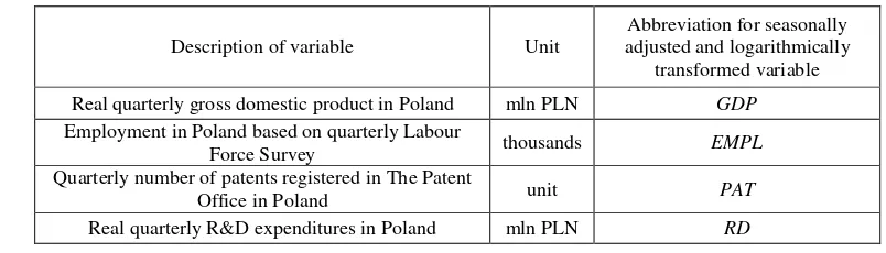
In this paper we use abbreviations for all the variables. Table 1 contains some initial
information:1
Description of variable Unit
Abbreviation for seasonally adjusted and logarithmically
transformed variable Real quarterly gross domestic product in Poland mln PLN GDP
Employment in Poland based on quarterly Labour
Force Survey thousands EMPL Quarterly number of patents registered in The Patent
[image:10.595.90.492.151.266.2]Office in Poland unit PAT Real quarterly R&D expenditures in Poland mln PLN RD
Table 1. Units, abbreviations and short description of examined variables.2
The first step in causality analysis is test for the stationarity of the variables under study. This
is the crucial precondition of traditional causality testing. Since it is unreasonable to expect
that GDP, the situation in the labour market and the performance of R&D sector in Poland
were generally changeless in the last decade, we may formulate the following:
Conjecture 1: All time series under study are nonstationary.
The probability of the existence of interdependencies between the technical progress related
variables (PAT and RD), employment and GDP is considerable in the light of the literature
overview presented in previous section. However, transitional countries like Poland are not
able to spend a similar amount of financial assets on R&D in comparison to other highly
developed OECD countries. Therefore, the impact of the relatively moderate spending on
R&D and patent applications on GDP in Poland is rather uncertain.
In the light of the literature the significant impact of patent applications on GDP is more
likely to exist since R&D outlays in Poland stem mainly from the state budget. The results
concerning contribution of public R&D investments to economic growth are unclear and in
some cases even controversial. As we cited in the introductory section, the EU applies as one
1
The authors would like to thank The Ministry of Finance of Poland, The Patent Office of Poland, The Central Statistical Office in Poland and Eurostat for their help in obtaining the dataset.
2
10
of the possible proxies of technical progress the number of researchers (scientists and
engineers). Behind this assumption there is a supposition that the more researchers there are
the more likely is the creation of inventions. In our opinion an inverse relation is also
probable: more inventions lead to a higher employment level not only in the R&D sector but
also in other sectors, especially in NTBFs. Since patents stand for the ‘output’ of the R&D
sector, an increasing number of patents may suggest a rise in the efficiency of investments in
the R&D sector and encourage government and firms to spend more money on further
research which implies increase of number of researchers. A more important supposition may
be that developing new technology implies the birth of new competitive firms (for example in
the ICT sector), which will employ new workers. This presumption is based on the
observation that unemployment in most countries with a high level of technology is low.
Therefore, we formulate a hypothesis concerning the role of patents in the growth of the
Polish economy and employment in the form:
Conjecture 2: There is a significant causal impact of the number of patents on GDP and
employment in the Polish economy in the short and long run.
Economic theory (production functions) predicts a dependence between labour input and
production output both in the short and long run. Therefore, by analogy, one can presume the
existence of causality between these two variables in the Granger sense. Since this
dependence is usually expressed by monotone increasing functions (with respect to
employment) feedback – mutual Granger causality between employment and GDP – can be
expected. Moreover, one can expect that the higher the employment in the whole economy,
the higher the employment in the R&D sector and the last fact implies the necessity of higher
11
Conjecture 3: There are some long run (short run) causalities between employment and
GDP (changes in employment and changes in GDP). Moreover, employment causes
changes in R&D outlays.
It is the common view in the literature based on empirical results that patents (by definition a
measure of innovations) contribute to economic growth. The existence of a connection
between PAT and RD can be justified theoretically by taking into account that the PAT time
series stands for the output of R&D investments (RD). This could be especially true in the
case of Poland, where most registered patents result from research supported by the
government.
Therefore, an indirect impact of R&D on GDP can be expected. In addition, R&D outlays
support the growth of human capital, which according to economic theory contributes to GDP
growth. In view of these facts, and results reported by some previous contributions related to
R&D–GDP links we formulate hypothesis 4 in the form:
Conjecture 4: There are linear and nonlinear Granger causalities from R&D expenditure to
GDP in Poland.
However, as stressed in the reviewed literature the empirical results concerning impact of
R&D on GDP are not uniform. In some empirical studies this impact is just neglected,
especially the effect of government R&D spending. Moreover, in some contributions it is
reported that registered patents are a causal factor for R&D, but not vice versa. This might be
justified by the assumption that patents are proofs of the efficiency of researchers and R&D
institutions. The more patents the more incentives in the future to invest in R&D by both the
government and private firms. This may be the case especially for developing or emerging
economies (like Poland) where only low or moderate financial assets can be invested in R&D.
12
Conjecture 5: There is a causal relationship running from the number of registered patents
to R&D outlays.
The hypotheses listed above will be tested by some recent causality tests. The details of the
testing procedures will be shown later. The test outcomes depend to some extent on the
testing methods applied, thus testing the robustness of empirical findings is one of our main
goals. Before describing the methodology, in the next section we will characterize the time
series included in our sample.
4. The dataset and its properties
The first part of this section contains a description of the applied dataset. In subsection 4.2 the
stationarity properties of all the time series are examined. The identification of the orders of
integration of the time series under study is a crucial stage of causality analysis.
4.1. Description of the dataset
The chosen dataset includes quarterly data on GDP, R&D outlays, the number of patents
registered in The Patent Office of Poland and employment in Poland in the period Q1 2000 –
Q4 2009. Thus, our dataset contains 40 observations. In order to remove the impact of
inflation we calculated GDP at constant prices (year 2000).
The Central Statistical Office in Poland presents original data on R&D expenditure only
on an annual basis. Therefore, in order to estimate the value of quarterly expenditures one is
forced to use a suitable procedure for dividing the overall (annual) outlays. In this paper we
used the following formula to calculate the estimates of quarterly R&D expenditure:
( )
(1 ) (1 )
4
x x
x x x x x
q q
x x x x x x x
q x x
SHE INV
RD GP GCE BP BCE
RD RD GP GCE RD BP BCE
SHE INV
⋅ + ⋅
= + ⋅ ⋅ ⋅ − + ⋅ ⋅ ⋅ − (1)
where:3
3
13
x q
RD – R&D expenditures in quarter q in year x (q∈{1, 2,3, 4}, x∈{2000, 2001,...., 2009});
x
RD – overall R&D expenditures in year x;
x
GP – share of government expenditures in R&D expenditures in year x;
x
BP – share of business (private) expenditures in R&D expenditures in year x;
x
GCE – share of current expenditures in government expenditures in R&D in year x;
x
BCE – share of current expenditures in business expenditures in R&D in year x; 4
x q
SHE – expenditures on science and higher education in quarter q in year x;
x
SHE – overall expenditures on science and higher education in year x;
x q
INV – investment outlays for fixed assets in quarter q in year x;
x
INV – overall investment outlays for fixed assets in year x.5
As we can see, the first component of the sum on the right side of equation (1) is exactly the
same for each quarter of year x. This fact reflects the assumption that current expenditures,
like labour costs, energy and fuel costs, are generally constant over a year.6 The second and
third components represent the quarter dependent parts of R&D expenditure. We applied
expenditures on science and higher education as well as investment outlays for fixed assets as
the most suitable weights for the government and private components, respectively.
Since each variable used was characterized by significant quarterly seasonality, and this
feature often leads to spurious results in causality analysis, the X–12 ARIMA procedure
(which is currently used by the U.S. Census Bureau for seasonal adjustment) of Gretl software
was applied to adjust each variable. Finally, each seasonally adjusted variable was
4 x
GP , x
BP , GCEx and BCEx lie between 0 and 1. Moreover, GPx+BPx =1 for all x since R&D outlays are either public or private.
5
The Central Statistical Office and Ministry of Finance provides data on expenditure expressed in current prices. However, all the time series of expenditures ( x
RD , x
q
SHE ,SHEx, x q
INV ,INVx) are expressed in constant prices of
year 2000 (due to the application of the inflation rate). Moreover, since data on investment outlays is presented by the Central Statistical Office only three times a year (first half–year, third quarter, fourth quarter) we assumed that INV1x=INV2x for all x.
6
When this paper was being prepared the annual report Science and technology in Poland in 2009 was still in production, thus it was impossible to get the 2009
RD , GP2009, 2009
BP , GCE2009, BCE2009 data directly from Central Statistical Office in Poland. However, for the sake of comparability with a model based on number of patents (it used data from 2009) we estimated quarterly R&D expenditures in 2009 using Eurostat data ( 2009
RD ,
2009
GP and 2009
BP were attainable in this office). However, exact data on GCE2009 and BCE2009 was unattainable even in Eurostat databases, thus we used forecasts based on simple linear trend models estimated for
x
14
transformed into logarithmic form, since this Box–Cox transformation may stabilize variance
and therefore improve the statistical properties of the data, which is especially important for
parametric tests.
The important point that distinguishes our paper from previous contributions on
technological progress and economic growth is that we applied (less aggregated) quarterly
data. This is partly because the data necessary covered only the recent few years and therefore
a causality analysis based on annual data could not have been carried out due to lack of
degrees of freedom.Moreover, as shown in some papers (Granger et al., 2000) the application
of lower frequency data (such as annual) may seriously distort the results of Granger causality
analysis because some important interactions may stay hidden.
The originality of this paper is also related to another important fact. As far as the authors
know this is the first study which analyses dynamic interactions between technological
progress and GDP in Poland, which is a leading country in the CEE region. The lack of
reliable datasets of sufficient size is a common characteristic of most of post–Soviet
economies and this can indeed be a serious problem for the researcher. However, the
application of recent quarterly data and modern econometric techniques (described in section
5) provided a basis for conducting this leading research for one of the transitional European
economies.
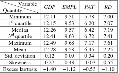
[image:15.595.201.397.622.743.2]The initial part of our analysis contains some descriptive statistics of all the variables.
Table 2 contains suitable results:
Variable
Quantity GDP EMPL PAT RD Minimum 12.11 9.51 5.78 7.00 1st quartile 12.15 9.53 6.20 7.07 Median 12.26 9.57 6.42 7.19 3rd quartile 12.41 9.63 6.72 7.41 Maximum 12.49 9.68 7.17 7.61 Mean 12.28 9.58 6.45 7.25 Std. deviation 0.12 0.09 0.34 0.20 Skewness 0.27 0.48 –0.03 0.55 Excess kurtosis –1.40 –1.12 –0.53 –1.10
15
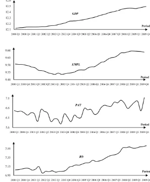
In order to conduct a comprehensive preliminary analysis the charts for all the variables under
[image:16.595.142.439.132.492.2]study should also be analyzed. The following figure contains suitable plots:
Figure 1. Plots of the time series.
In years 2000–2009 there was relatively stable development of the Polish economy since
GDP exhibited an upward tendency. One cannot forget that the Polish economy was one of
the few that managed to avoid an undesirable impact of the crisis of 2008. However, after
September 2008 one could observe the beginning of slight slowdown in the rate of growth of
the Polish economy. For EMPL in the analyzed period there was a stable rise between 2003
and 2008. However, slight drops were also observed before 2003 and after the crisis of
September 2008. Similar regularities were also observed for R&D expenditures. Between
16
financial crisis of 2008 definitely caused an inhibition of the rate of growth of these
expenditures. Finally, one should note that the PAT time series also exhibits an upward
tendency. However, the slope of the trend line is relatively low in this case. Moreover, in
comparison to other time series PAT is least smooth.7
The descriptive analysis of the time series included in our dataset will be extended in the
next subsection by stationarity testing. This is a crucial stage of causality analysis.
4.2. Stationarity properties of the dataset
In the first step of this part of research we conducted an Augmented Dickey–Fuller (ADF)
unit root test.8 However, the application of the ADF test involves two serious problems.
Firstly, the outcomes of this test are relatively sensitive to an incorrect establishment of lag
parameter. Secondly, the ADF test tends to under–reject the null hypothesis pointing at
nonstationarity too often.9 Therefore, the Kwiatkowski–Phillips–Schmidt–Shin (KPSS) test
was conducted to confirm the results of the ADF one. In contrast to the ADF test the null
hypothesis of a KPSS test refers to the stationarity of the time series.
Since it is possible that two unit root tests lead to contradictory conclusions, a third test
must be applied to make a final decision about the stationarity of time series. In this paper we
additionally applied the Phillips–Perron (PP) test, which is based on a nonparametric method
of controlling for serial correlation when testing for a unit root. The null hypothesis once
again refers to nonstationarity.
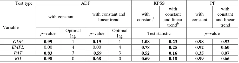
Table 3 contains the results of the stationarity analysis. Bold face indicates finding
nonstationarity at a 5% level:
7
The range and variation of PAT are highest of all the time series. One may easily imagine a 50% drop (or rise) in the number of patents in quarters q and q+1. However, it is impossible to observe such a phenomenon for GDP, employment or R&D expenditures.
8
Before conducting the test, the maximal lag length was set at a level of 6 and then the information criteria (namely, the AIC, BIC and HQ) were applied to choose the optimal lag.
9
17
Test type
Variable
ADF KPSS PP
with constant with constant and linear trend
with constanta
with constant and linear
trendb
with constant
with constant and linear
trend
p–value Optimal
lag p–value
Optimal
lag Test statistic p–value
GDP 0.99 1 0.19 1 1.08 0.23 0.98 0.52
EMPL 0.00 4 0.00 4 0.78 0.25 0.92 0.60
PAT 0.83 3 0.59 3 0.52 0.16 0.35 0.07
[image:18.595.69.529.112.233.2]RD 0.98 0 0.68 0 0.69 0.18 0.99 0.66
Table 3. Results of stationarity analysis.
a
critical values: 0.347 (10%), 0.463 (5%), 0.739 (1%).
b
critical values: 0.119 (10%), 0.146 (5%), 0.216 (1%).
An analysis of the outcomes presented in table 3 shows that all time series were found to be
nonstationary around constant at a 5% level.10 Therefore, conjecture 1 should be accepted.
Some further calculations (conducted for first differences) confirmed that all variables under
study are I(1).11
5. Methodology
In this paper several econometric tools were applied to test for both linear and nonlinear
Granger causality between GDP and technological progress in Polish economy. The main part
of our research was conducted in two three–dimensional variants, each of which involved
GDP, EMPL and one variable related to technological progress (that is PAT or RD).
5.1. Linear short and long run Granger causality tests
Since the concept of Granger (1969) causality is well known and has been commonly applied
in previous empirical studies we will not explain it in detail. By and large, this idea is used to
examine whether a knowledge of the past and current values of one stationary variable is
helpful in predicting the future values of another one or not. Stationarity is a crucial
precondition for standard linear Granger causality tests. Nonstationarity of the time series
10
All three tests pointed at nonstationarity for every analyzed time series except for EMPL. In this case nonstationarity was confirmed by two of three conducted tests.
11
18
under study may lead to misleading conclusions by a traditional linear causality test. This
phenomenon has been investigated in previous empirical (Granger and Newbold, 1974) and
theoretical (Phillips, 1986) deliberations. Since all the variables were found to be I(1) we
applied three econometric methods suitable for testing for linear short and long run Granger
causality in this context, namely, a traditional analysis of the vector error correction model
(VECM), the sequential elimination of insignificant variables in VECM and the Toda–
Yamamoto method.
A cointegration analysis (based on the estimation of a VEC model) may be performed for
variables which are integrated in the same order. As shown by Granger (1988) the existence
of cointegration implies long run Granger causality in at least one direction. To establish the
direction of this causal link one should estimate a suitable VEC model and check (using a t–
test) the statistical significance of the error correction terms. Testing the joint significance
(using an F–test) of lagged differences provides a basis for short run causality investigations.
However, causality testing based on the application of an unrestricted VEC model has got
a serious drawback. Namely, in practice it is often necessary to use a relatively large number
of lags in order to avoid the consequences of the autocorrelation of residuals. On the other
hand, a large number of lags may lead to a significant reduction in the number of degrees of
freedom, which in turn has an undesirable impact on test performance, especially for small
samples. Moreover, testing for linear causality using a traditional Granger test often suffers
because of possible multicollinearity. Therefore, in order to test for short and long run linear
Granger causality a sequential elimination of insignificant variables was additionally applied
for each VECM equation separately. At each step of this procedure the variable with the
highest p–value (t–test) was omitted until all remaining variables have a p–value no greater
than a fixed value (in this paper it was 0.10). The Reader may find more technical details of
19
Another approach for testing for linear Granger causality was formulated by Toda and
Yamamoto (1995). This method has been commonly applied in recent empirical studies (see,
for example, Mulas–Granados and Sanz, 2008) since it is relatively simple to perform and
free of complicated pretesting procedures, which may bias the test results, especially when
dealing with nonstationary variables. The most important feature of the Toda–Yamamoto
(TY) approach is the fact that this procedure is applicable even if the variables under study are
characterized by different orders of integration.12 In such cases a standard linear causality
analysis cannot be performed by the direct application of a basic VAR or VEC model. On the
other hand, differencing or calculating the growth rates of some variables allows the use of
the traditional approach, but it may also cause a loss of long run information and lead to
problems with the interpretation of test results.
The idea behind the Toda and Yamamoto approach for causality testing is relatively
simple as it is just a modification of the standard Wald test. To shed light on this procedure let
us assume that the true DGP is an n–dimensional VAR(p) process. If the order of this process
(p) is unknown, it may be established with the help of standard model selection criteria (for
more details see Paulsen, 1984). In the next step the highest order of integration of all the
variables in the VAR model (let d denote this value) should be established. Finally, the
augmented VAR(p+d) model should be fitted to the dataset. A Toda–Yamamoto test statistic
is just a standard Wald test applied to test null restrictions only for the first p lags of the
augmented VAR model. If some typical modelling assumptions (for instance, the error term
being white noise) hold true for the augmented model then the test statistic has the usual
asymptotic 2
( )p
χ distribution (Toda and Yamamoto, 1995). However, since we dealt with
relatively small samples we applied the TY test statistic in its asymptotically F–distributed
variant, which performs better for small samples (Lütkepohl, 1993).
12
20
The application of these parametric methods has got two serious drawbacks. Firstly, if
suitable modelling assumptions do not hold the application of asymptotic theory may lead to
spurious results. Secondly, regardless of the modelling assumptions, the distribution of the
test statistic may be significantly different from an asymptotic pattern when dealing with
extremely small samples. The application of the bootstrap technique provides one possible
way of overcoming these difficulties. Bootstrapping is used for estimating the distribution of a
test statistic by resampling data. It seems reasonable to expect that the bootstrap procedure
does not require such strong assumptions as parametric methods, since the estimated
distribution depends only on the available dataset. However, bootstrapping is likely to fail in
some specific cases and therefore cannot be treated as a perfect tool for solving all possible
model specification problems (Horowitz, 1995).
In order to minimize the undesirable influence of heteroscedasticity, the bootstrap test was
based on resampling leveraged residuals.13 Academic discussion on the establishment of the
number of bootstrap replications has attracted considerable attention in recent years
(Horowitz, 1995). In this paper the recently developed procedure of establishing the number
of bootstrap replications presented by Andrews and Buchinsky (2000) was applied. In all
cases we aimed to choose such a value of number of replicationswhich would ensure that the
relative error of establishing the critical value (at a 10% significance level) would not exceed
5% with a probability equal to 0.95.14
5.2. Nonlinear Granger causality test
In general, the application of nonlinear methods in testing for Granger causality is based on
two facts. First, as shown in some papers (see, for example, Brock, 1991) the traditional linear
Granger causality test tends to have extremely low power in detecting certain kinds of
13
The detailed description of resampling procedure applied in this paper may be found in Hacker and Hatemi (2006).
14
21
nonlinear causal interrelations. Second, linear methods are mainly based on testing the
statistical significance of suitable parameters only in a mean equation, thus causality in any
higher–order structure (such as variance) cannot be explored (Diks and DeGoede, 2001).
In this paper we applied the nonlinear causality test proposed by Diks and Panchenko
(2006). We applied some typical values of the technical parameters of this method, which
have been commonly used in previous papers (see, for example, Diks and Panchenko (2006),
Gurgul and Lach (2010)). We set up the bandwidth (denoted as ε) at a level of 0.5, 1 and 1.5
while the common lag parameter (denoted as l) was set at the order of 1 and 2. The Reader
may find a detailed description of the role of these technical parameters and the form of test
statistic in Diks and Panchenko (2006).15
Since previous studies (Diks and Panchenko, 2006) provided evidence that the presence of
heteroscedasticity leads to over–rejection of the discussed nonlinear test, we additionally
decided to test all examined time series for the presence of various heteroscedastic structures
(using, inter alia, White’s test and a Breusch–Pagan test).
6. Empirical results
In this section the results of short and long run linear Granger causality analysis as well as the
outcomes of nonlinear causality tests are presented. The main goal of these empirical
investigations was to examine the structure of the dynamic relationships between different
measures of technological progress and GDP in Poland in the period Q1 2000 – Q4 2009. As
already mentioned, the main part of the research was performed in a three–dimensional
framework, since fluctuations in employment may have a significant impact on the structure
of technology–GDP links.16
15
We applied Diks and Panchenko’s (2006) nonlinear procedure using all practical suggestions presented in Gurgul and Lach (2010).
16
22
6.1. Number of patents and GDP
Since PAT, GDP and EMPL were all found to be I(1) we first performed a cointegration
analysis for these variables. We analyzed the possibilities listed in Johansen (1995) to specify
the type of deterministic trend. In view of the results presented in subsection 4.2 (no trend–
stationarity) the Johansen’s third case was assumed, that is the presence of a constant in both
the cointegrating equation and the test VAR. In the next step, the information criteria (namely,
AIC, BIC, HQ) were applied to establish the appropriate number of lags. The final lag length
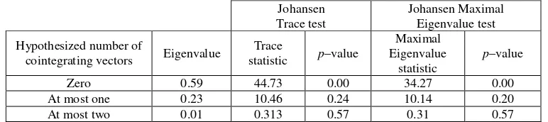
was set at a level of 5.17 The following table contains the results of Johansen cointegration
tests:
Johansen Trace test
Johansen Maximal Eigenvalue test Hypothesized number of
cointegrating vectors Eigenvalue
Trace
statistic p–value
Maximal Eigenvalue
statistic
[image:23.595.105.491.337.423.2]p–value Zero 0.59 44.73 0.00 34.27 0.00 At most one 0.23 10.46 0.24 10.14 0.20 At most two 0.01 0.313 0.57 0.31 0.57
Table 4. Results of cointegration analysis for PAT, GDP and EMPL variables.
One can see that both variants of Johansen test provided solid evidence (at all typical
significance levels) for claiming that for these variables the dimension of cointegration space
is equal to one. Moreover, the hypothesis that the smallest eigenvalue is equal to zero was
accepted (last row of table 4), which additionally validates the results of the previously
performed unit root tests.18 Next, we estimated a suitable VEC model assuming 4 lags (for
first differences) and one cointegrating vector. Table 5 contains p–values obtained while
17
We set the maximal lag length (for levels) at a level of 6. BIC criterion pointed at one lag, however the results of Ljung–Box Q–test confirmed that in the case of one lag residuals were significantly autocorrelated, which in turn may lead to serious distortion of the results of the causality analysis.
18
23
testing for linear short and long run Granger causality using an unrestricted VEC model and
the sequential elimination of insignificant variables:19
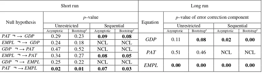
Short run Long run
Null hypothesis
p–value
Equation
p–value of error correctioncomponent
Unrestricted Sequential Unrestricted Sequential
Asymptotic Bootstrapa
Asymptotic Bootstrapa
Asymptotic Bootstrapa
Asymptotic Bootstrapa
PAT GDP 0.29 0.23 0.09 0.08
GDP 0.11 0.08 0.02 0.00
EMPL GDP 0.24 0.18 NCL NCL
GDP PAT 0.47 0.52 NCL NCL
PAT 0.51 0.46 NCL NCL
EMPL PAT 0.34 0.27 0.08 0.05
GDP EMPL 0.25 0.22 NCL NCL
EMPL 0.00 0.00 0.00 0.00
[image:24.595.78.523.126.252.2]PAT EMPL 0.02 0.01 0.07 0.03
Table 5. Analysis of causal links between PAT, GDP and EMPL variables (VEC models). a Number of bootstrap replications established using Andrews and Buchinsky
(2000) method varied between
1469 and 2699.
The results obtained for the unrestricted VEC model provided a basis for claiming that PAT
Granger caused EMPL in the short run in the period under study. On the other hand, the
sequential elimination of insignificant variables led to the conclusion that in the short run
there was feedback between these variables. Moreover, PAT was found to Granger cause
GDP. It is worth mentioning that all these results were found in asymptotic– and bootstrap–
based research variants.
In all the research variants (except for the asymptotic–based variant in an unrestricted
model) the error correction component was found to be significant in the GDP and EMPL
equations, which provides a basis for claiming that for GDP and employment there was
feedback in the long run. Furthermore, the number of patents was found to Granger cause
GDP and EMPL in the long run.
For the sake of comprehensiveness we additionally applied the Toda–Yamamoto approach
for testing for causal effects between PAT, GDP and EMPL. The outcomes of the TY
19
Through this paper the notation ‘x y’ is equivalent to ‘x does not Granger cause y’. Moreover, the symbol ‘NCL’ is the abbreviation of ‘No coefficients left’. Finally, bold face always indicates finding a causal link in a particular direction at a 10% significance level.
¬ → ¬ → ¬ →
¬ → ¬ → ¬ →
24
procedure provided no basis for claiming that linear causality runs in any direction for the
variables (at a 10% significance level), thus we do not present them in a separate table.
In the last step of the causality analysis, a nonlinear test was performed for the residuals
resulting from all linear models, namely, the residuals of unrestricted VECM, the residuals
resulting from individually (sequentially) restricted equations and the residuals resulting from
the augmented VAR model applied in the Toda–Yamamoto method.20 For each combination
of ε and l three p–values are presented according to the following rule:
p–value for residuals of unrestricted VEC model
p–value for residuals of sequentially restricted equations
p–value for residuals of TY procedure
Since in all examined cases no significant evidence of heteroscedasticity was found, no
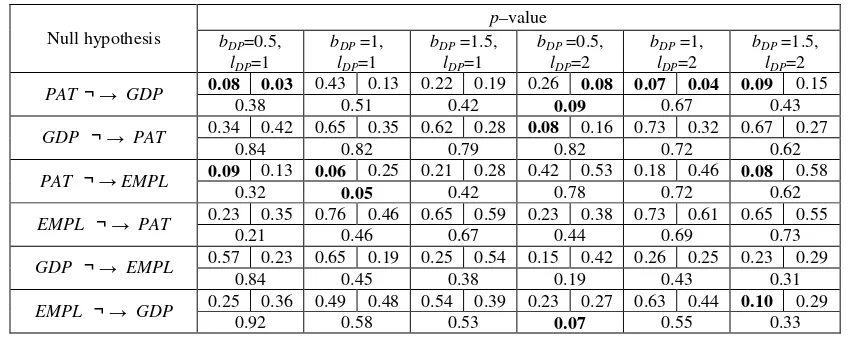
filtering was used. Following table contains suitable results:
Null hypothesis
p–value
bDP=0.5,
lDP=1
bDP =1,
lDP=1
bDP =1.5,
lDP=1
bDP =0.5,
lDP=2
bDP =1,
lDP=2
bDP =1.5,
lDP=2
PAT GDP 0.08 0.03 0.43 0.13 0.22 0.19 0.26 0.08 0.07 0.04 0.09 0.15
0.38 0.51 0.42 0.09 0.67 0.43
GDP PAT 0.34 0.42 0.65 0.35 0.62 0.28 0.08 0.16 0.73 0.32 0.67 0.27
0.84 0.82 0.79 0.82 0.72 0.62
PAT EMPL 0.09 0.13 0.06 0.25 0.21 0.28 0.42 0.53 0.18 0.46 0.08 0.58
0.32 0.05 0.42 0.78 0.72 0.62
EMPL PAT 0.23 0.35 0.76 0.46 0.65 0.59 0.23 0.38 0.73 0.61 0.65 0.55
0.21 0.46 0.67 0.44 0.69 0.73
GDP EMPL 0.57 0.23 0.65 0.19 0.25 0.54 0.15 0.42 0.26 0.25 0.23 0.29
0.84 0.45 0.38 0.19 0.43 0.31
EMPL GDP 0.25 0.36 0.49 0.48 0.54 0.39 0.23 0.27 0.63 0.44 0.10 0.29
[image:25.595.85.512.368.538.2]0.92 0.58 0.53 0.07 0.55 0.33
Table 6. Analysis of nonlinear causal links between PAT, GDP and EMPL variables
As one can see nonlinear causality running from PAT to GDP was confirmed by all nonlinear
tests (for residuals from unrestricted VECM feedback was even detected). Moreover, we
found strong support for claiming that there is nonlinear unidirectional causality from the
number of patents to employment. This was confirmed by an analysis of the residuals of
unrestricted VEC model and the residuals of the augmented model applied in the TY
procedure.
20
Since the structure of linear connections had been filtered out after an analysis of linear models, the residuals are believed to reflect strict nonlinear dependencies (Baek and Brock, 1992).
The results of all the met
number of patents registered in
of real GDP and employment
also be accepted. Moreover, th
completely different methods
with respective nonlinear tes
robustness when exposed to st
results of both econometric a
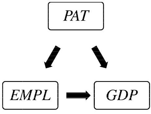
Therefore, we found that PAT
on employment). To summariz
[image:26.595.179.422.379.562.2]PAT, EMPL and GDP in the fo
Figure 2. The structu
We must remember that figure
EMPL and GDP, which was
causalities (the short run impac
also reported, but they were
applied in this paper. There is
they were found to be far less
25
ethods provided relatively strong support for
d in The Patent Office of Poland is a causal fac
nt both in the short and long run. Therefore, c
, this conclusion, in general, was confirmed by
ds (a two–stage analysis of the VEC model and
tests), which validates this major conclusion
statistical tools. Another important conclusion
c approaches is the causal influence of emp
AT causes GDP directly and indirectly (through
rize one may present the structure of causal dep
following figure:
cture of causal links between the PAT, EMPL a
ure 2 present the structure of causal dependen
as evidently supported by our empirical re
pact of employment on PAT, causality from GD
re not supported by the results of both econo
is no reason to treat these causal links as unim
significant than those presented in figure 2.
for claiming that the
factor for movements
, conjecture 2 should
by the results of two
and the TY approach
ion and confirms its
ion supported by the
ployment on GDP.
gh a causal influence
dependences between
and GDP.
encies between PAT,
results. Some other
GDP to EMPL) were
nometric procedures
26
6.2. R&D expendituresand GDP
As in the previous case (subsection 6.1), in the first step cointegration analysis was carried out
for the RD, GDP and EMPL variables.21 The following table contains the results of
cointegration tests performed under the assumption of Johansen’s third variant and 4 lags (for
variables in first differences):
Johansen Trace test
Johansen Maximal Eigenvalue test Hypothesized number of
cointegrating vectors Eigenvalue
Trace
statistic p–value
Maximal Eigenvalue
statistic
[image:27.595.101.491.208.297.2]p–value Zero 0.41 34.45 0.01 18.60 0.09 At most one 0.36 15.95 0.04 15.95 0.02 At most two 0.00 0.00 0.97 0.00 0.97
Table 7. Results of cointegration analysis for the RD, GDP and EMPL variables.
Regardless of the type of test used the dimension of cointegration space was found to be equal
to two (at 10% significance level). As in the previous case (table 4) the nonstationarity of all
variables was once again confirmed. In the next step we estimated a suitable VEC model
assuming 4 lags (for first differences) and two cointegrating vectors.22 Table 8 contains p–
values obtained while testing for linear short and long run Granger causality using
unrestricted VEC model and the sequential elimination of insignificant variables:
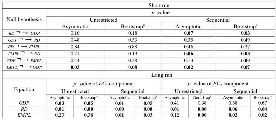
Short run Null hypothesis
p–value
Unrestricted Sequential
Asymptotic Bootstrapa Asymptotic Bootstrapa
RD¬ → GDP 0.16 0.18 0.07 0.03
GDP ¬ → RD 0.48 0.33 0.35 0.49
RD¬ →EMPL 0.84 0.88 0.46 0.37
EMPL¬ →RD 0.21 0.19 0.06 0.03
GDP¬ →EMPL 0.44 0.38 0.13 0.09
EMPL¬ →GDP 0.03 0.08 0.02 0.07
Long run Equation
p–value of EC1 component p–value of EC2 component
Unrestricted Sequential Unrestricted Sequential
Asymptotic Bootstrapa Asymptotic Bootstrapa Asymptotic Bootstrapa Asymptotic Bootstrapa
GDP 0.03 0.05 0.01 0.05 0.41 0.38 0.38 0.67
RD 0.01 0.00 0.00 0.00 0.01 0.00 0.06 0.04
EMPL 0.23 0.38 0.01 0.03 0.12 0.06 0.02 0.02
Table 8. Analysis of causal links between RD, GDP and EMPL variables (VEC model). aNumber of bootstrap replications established using the Andrews and Buchinsky
(2000) method varied between
1589 and 2939.
21
The preliminary part of cointegration analysis (specification of the type of deterministic trend, lag selection procedure) was performed in exactly the same way as in the case of PAT, EMPL and GDP variables
22
[image:27.595.75.518.487.682.2]27
As we can see, this time the results obtained for the unrestricted VEC model provided a basis
for claiming that there is unidirectional short run causality running from employment to GDP.
No other short run dependencies were found for the unrestricted model, although in two cases
(testing causality from RD to GDP and from EMPL to RD) the p–values were relatively small.
The results obtained for sequentially restricted equations confirmed the existence of short run
causality from EMPL to GDP. However, this time causality from RD to GDP and from EMPL
to RD was found to be significant at a 10% level. On the other hand, both methods applied to
the VEC model provided relatively solid evidence for the existence of long run feedback
between quarterly R&D expenditures and employment as well as between RD and GDP. The
long term impact of GDP on EMPL was found to be statistically significant only after the
sequential elimination.
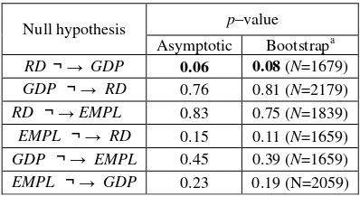
As in subsection 6.1, the Toda–Yamamoto approach was also applied to the RD, GDP and
EMPL variables. The following table contains the outcomes of the TY procedure:
Null hypothesis p–value Asymptotic Bootstrapa
RD GDP 0.06 0.08 (N=1679)
GDP RD 0.76 0.81 (N=2179)
RD EMPL 0.83 0.75 (N=1839)
EMPL RD 0.15 0.11 (N=1659)
GDP EMPL 0.45 0.39 (N=1659)
[image:28.595.198.397.434.543.2]EMPL GDP 0.23 0.19 (N=2059)
Table 9. Analysis of causal links between the RD, GDP and EMPL variables (TY approach).
a Parameter N denotes the number of bootstrap replications established according to the Andrews and Buchinsky
(2000) procedure.
The analysis of outcomes presented in table 9 leads to the conclusion that R&D expenditures
Granger cause GDP. Although the p–values obtained while testing for causality in other
directions were greater than 0.10, the dynamic impact of EMPL on RD was found to be
‘almost’ significant (p–value at the level of 0.11 in the bootstrap variant).
The last stage of causality analysis was based on the application of Diks and Panchenko’s
nonlinear test. As in the previous case, the test was performed for the time series of residuals.
¬ → ¬ → ¬ →
¬ → ¬ →
28
Since no significant evidence of heteroscedasticity was found, no filtering was used. Table 10
presents the p–values obtained while testing for nonlinear Granger causality between RD,
GDP and EMPL. The test outcomes are presented according to the rule preceding presentation
of table 6:
Null hypothesis
p–value
bDP=0.5,
lDP=1
bDP =1,
lDP=1
bDP =1.5,
lDP=1
bDP =0.5,
lDP=2
bDP =1,
lDP=2
bDP =1.5,
lDP=2
RD GDP 0.48 0.53 0.44 0.28 0.61 0.36 0.43 0.53 0.26 0.47 0.34 0.84
0.69 0.34 0.31 0.72 0.29 0.23
GDP RD 0.69 0.43 0.17 0.27 0.58 0.73 0.81 0.62 0.71 0.53 0.81 0.76
0.71 0.21 0.55 0.62 0.28 0.45
RD EMPL 0.81 0.75 0.74 0.67 0.65 0.62 0.36 0.48 0.43 0.29 0.49 0.71
0.42 0.41 0.61 0.50 0.35 0.43
EMPL RD 0.08 0.19 0.06 0.32 0.21 0.37 0.22 0.72 0.21 0.63 0.47 0.59
0.09 0.34 0.44 0.21 0.27 0.29
GDP EMPL 0.24 0.83 0.92 0.72 0.31 0.49 0.81 0.67 0.55 0.42 0.23 0.44
0.36 0.18 0.28 0.31 0.06 0.37
EMPL GDP 0.27 0.57 0.73 0.69 0.63 0.31 0.14 0.38 0.63 0.46 0.71 0.52
0.30 0.63 0.08 0.57 0.09 0.15
Table10. Analysis of nonlinear causal links between the RD, GDP and EMPL variables.
This time nonlinear causality running from EMPL to RD was confirmed by all but one test
(for residuals from sequentially restricted VECM no nonlinear causality was reported).
Moreover, analysis of the residuals from the augmented model applied in the TY procedure
provided a basis for claiming that there is nonlinear feedback between GDP and EMPL.
Generally, the results of all the methods provided relatively strong support for claiming
that R&D expenditure is a causal factor for movements of real GDP both in the short and long
run, which supports conjecture 4. Moreover, employment was found to Granger cause RD and
GDP, which additionally provides a basis for accepting conjecture 3. These conclusions, in
general, were once again confirmed by the results of the two econometric methods applied,
which is especially important in terms of the validation and robustness of the empirical
results. To summarize one may present the structure of causal dependences between RD,
EMPL and GDP in the following figure:
¬ →
¬ →
¬ →
¬ →
¬ →
Figure 3. The struct
We should once again underl
between RD, EMPL and GDP
other causalities (in opposite
(mostly in the long term). Ho
procedures applied in this pape
6.3. Out
The results presented in sub
conjecture 5 is true, in other
patents to R&D expenditure (i
RD). This conclusion is of grea
sector (researchers, politicians
different econometric models.
additionally performed an anal
which involves both these vari
29
ucture of causal links between the RD, EMPL an
erline that figure 3 present the structure of c
P which was evidently supported by our empi
te directions to those presented in figure 3) w
However, these results were not confirmed by
aper, which leads to some doubt about their exis
utlays on R&D versus number of patents
subsections 6.1 and 6.2 provided evidence
er words there is Granger causality running fr
e (indirectly, as PAT causes employment and e
reat importance for a number of social groups r
ans, investors). However, it is based on result
ls. Therefore, in order to confirm or contradi
nalysis of causal dependences between PAT and
ariables.
and GDP.
f causal dependences
pirical results. Some
) were also reported
by both econometric
xistence.
e for claiming that
from the number of
d employment causes
s related to the R&D
ults obtained for two
adict this finding we