LAN Tool: A GIS Tool for the Improvement of Digital Elevation Models Using Drainage Network Attributes

LAN Tool: A GIS Tool for the Improvement of Digital

Elevation Models Using Drainage Network Attributes

Alexandra Gemitzi1*, Odysseas Christou2

1

Department of Environmental Engineering, Faculty of Engineering, Democritus University of Thrace, Xanthi, Greece

2

Geoinfo Cyprus Limited, Larnaca, Cyprus Email: *[email protected], [email protected]

Received March 24, 2013; revised April 24, 2013; accepted May 24,2013

Copyright © 2013 Alexandra Gemitzi, Odysseas Christou. This is an open access article distributed under the Creative Commons Attribution License, which permits unrestricted use, distribution, and reproduction in any medium, provided the original work is properly cited.

ABSTRACT

Digital Elevation Models (DEMs) are constructed using altitude point data and various interpolation techniques. The quality and accuracy of DEMs depend on data point density and the interpolation technique used. Usually however, altitude point data especially in plain areas do not provide realistic DEMs, mainly due to errors produced as a result of the interpolation technique, resulting in imprecise topographic representation of the landscape. Such inconsistencies, which are mainly in the form of surface depressions, are especially crucial when DEMs are used as input to hydrologic modeling for impact studies, as they have a negative impact on the model’s performance. This study presents a Geo-graphical Information System (GIS) tool, named LAN (Line Attribute Network), for the improvement of DEM con-struction techniques and their spatial accuracy, using drainage network attributes. The developed tool does not alter the interpolation technique, but provides higher point density in areas where most DEM problems occur, such as lowland areas or places where artificial topographic features exist. Application of the LAN tool in two test sites showed that it provides considerable DEM improvement.

Keywords: Digital Elevation Model (DEM); Geographical Information Systems (GIS); Drainage Network; Spatial

Interpolation; Hydrologic Modeling

1. Introduction

Digital Elevation Models (DEMs) are numerical repre-sentations of areas on the earth’s surface produced ap-plying interpolation techniques on altitude point data. DEMs provide vital input to several scientific areas and have numerous applications, among others in telecom-munications, military services, location based services and environmental services. One of the most important applications of DEMs is their use in hydrologic modeling. As climate and land use changes have already brought serious impacts on local communities such as floods, droughts, soil erosion and pollution from point and non-point sources, scientists and decision makers are concerned on having realistic hydrologic models capable of simulating runoff, and sediment and nutrient loadings, in order to determine areas and ecosystems that are prone to be affected in the future.

The importance of DEM quality on hydrologic studies is already depicted by many researchers. Legleiter and

Kyriakidis [1], indicated the problems usually encoun-tered while constructing a DEM from a number of dis-crete altitude data points acquired through field survey and pointed out the fact that sophisticated methods of spatial prediction are no substitute for field data. The impact of DEM quality in hydrologic modeling, hazard modeling, stream network delineation, floodplain bound- aries is highlighted in many studies [2-6].

Much research is also focused on detecting and im-proving the accuracy of DEMs and comparative studies have been conducted on the accuracy of the results of various interpolation techniques [7-12]. Several tech-niques have been developed for error minimization and DEM improvement including data fusion and other so-phisticated techniques which however require the avail-ability of multi-source DEM products [13,14]. Other methods provide combination or adjustments of various interpolation models [15,16].

Early studies have dealt with the problem of improv-ing DEM quality usimprov-ing drainage enforcement algorithms incorporating stream line data. Chen et al. [17], presented

a comparative study of the drainage constrained methods, categorizing them in three main groups, i.e.: stream burning, surface fitting, and constrained-TIN algorithms. The stream burning algorithms apply a raster representa-tion of a vector stream network in order to capture known hydrological features into a DEM [18,19]. The most popular surface fitting algorithm was presented by Hutchinson [20], known as ANUDEM algorithm, in-tending to remove pits from DEMs. In this methodology, irregularly spaced elevation data points, streamline and contour line data are used together with a finite differ-ence interpolation technique. In the constrained TIN ap-proaches, TINs are used instead of square grid cells in the DEM. Recently, Zhou and Chen [21], presented the compound method, constructing a drainage-constrained TIN, optimized to keep the important terrain features and slope morphology. Such algorithms are mainly targeting at DEM generalization, acting as correctors to the already constructed DEM, by altering point altitude where nec-essary and utilizing a specific interpolation method each time. In that way, although all previously mentioned methods provided DEM improvements, they achieved it through reconfigurations of certain interpolation methods and therefore they focused on a specific interpolation method. However none of the known interpolation me- thods provide accurate predictions in all cases and the development of a DEM improvement methodology using a certain interpolation technique is quite restrictive. This paper presents a DEM improving methodology that works before any interpolation is attempted and aims at im- proving input data point density incorporating stream line data into the original altitude point data set without al- tering any of the existing data points. This is achieved by assigning automatically an altitude attribute to the river network points, based on the intersections of the river lines with the altitude contours and by interpolating addi- tional altitude points between intersection points. In that way, errors in the drainage network which are common due to artificial or even natural changes in topography, artificial drainage network construction, low density of point altitude data in lowland areas, or even errors pro-duced by the interpolation may well be eliminated. The major difference from the previously mentioned methods for DEM improvement is that the present tool does not alter any of the initially existing data points. As it acts prior to DEM construction, it is not dedicated to any in- terpolation method and therefore it provides greater fle- xibility for the user to choose any interpolation method fits better to the case study each time.

Legleiter and Kyriakidis [1], mentioned that root mean- square error of the predictions provided by interpolation methods is directly proportional to the spacing between surveyed cross-sections, even in a reconfigured channel with a relatively simple morphology. In this context and

because of the fact that the methodology presented herein provides higher density of point altitude data in the drainage network, it seems that it is a useful alternative for DEM improvement especially in cases where hydro-logic modeling is of prime interest.

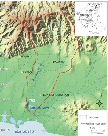
The methodology is demonstrated in two parts of the Vosvozis river basin, in northern Greece (Figure 1).

2. Materials and Methods

2.1. Study Area

The study area, Vosvozis river basin, located in northern Greece covers 357 km2 (Figure 1). The southern lowland part is an agricultural area. The river course in that part has undergone many interventions, thus changing com-pletely the natural drainage pattern during the last dec-ades. Moreover, many artificial drainage tiles have been constructed. The northern mountainous part is a forested area that has remained largely unchanged.

2.2. Methodology and Theoretical Background

LAN tool was developed using the Mapinfo MapBasic programming language and works as a seamless add on tool within Mapinfo Professional ver. 7 or later. The idea is to provide a higher point density as predefined by the user. In our case linear objects represent the drainage network of an area. Nevertheless, the same methodology

may well be applied for other linear features, e.g. for the road network of an area, where enhanced point density is required.

In any case the user is prompted to provide two vector files, one with the altitude contours that will be used for the construction of the DEM and one with the linear ob-jects that will be used for the production of new altitude data points (Figure 2).

Subsequently, the user chooses the required point dis-tance to be produced on the linear objects (Figure 3).

Then LAN tool detects all intersecting points of the given linear objects with the altitude contours as shown in Figure 4 and creates nodes at those points. In order to detect those intersections the well known sweep line al-gorithm is used [22]. This alal-gorithm uses a sweeping vertical line from left to right in order to detect the k in-tersections of n line segments. The status of this sweep line changes constantly as the line moves and is defined by the set of segments intersecting it each time. The sweep line changes its status every time it passes an end point of a line segment or an intersecting point. As all data points are processed in sorted order the intersections are also provided in sorted order too. The advantage of this algorithm is that unlike conventional intersection search algorithms that require O(n2) time, the sweep line algorithm requires O((n + k)logn) time to run and there-fore it provides a fast and robust way to define intersec-tion points.

Figure 2. Selection of input files within LAN tool.

Figure 3. Selection of input parameters for LAN tool.

Figure 4. Intersection of altitude contour lines with river network.

Altitude values are assigned to those intersecting nodes based on the intersecting contour. Following, each line segment between those newly produced nodes is divided into equally spaced parts, and a new node is created for each one, according to the user predefined maximum required node distance. Then, LAN tool assigns altitude values to those new nodes performing either linear or cubic spline interpolation as shown on Figure 5, based on user’s choice.

Linear interpolation fits a different linear function be-tween each pair of existing data points, i.e., nodes of known altitude and returns the value of the relevant func-tion at the interpolated points. The cubic spline fits a dif-ferent cubic function between each pair of existing data points. Figure 5 shows an example of the application of those two different techniques. The produced nodes are spaced at 5 m. It is true that the cubic spline produces a more realistic representation of the topography; however when the distance between original nodes is small (sec-ond and third point on Figure 4) then the two methods produce almost identical results. Taking into account the fact that linear interpolation is much faster, it depends on the user to choose the optimum method, based on the density of the original data points. After the new nodes have been assigned altitude values, LAN tool creates a new vector file containing all original and newly pro-duced data points, in order to be used for DEM construc-tion using convenconstruc-tional interpolaconstruc-tion techniques.

It should be noted herein that also in the case of low-land areas where pits are often a problem when applying a hydrologic model, LAN tool is a useful alternative to pit removal algorithms used in most commercial GIS software, after DEM construction.

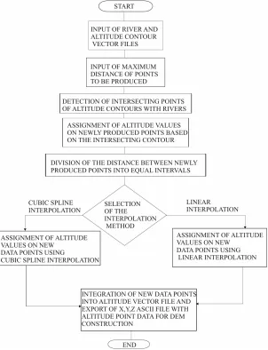
The flow chart of the developed software is shown on Figure 6.

Figure 5. Cross sectional diagram of a river showing the results of linear and cubic spline interpolation.

Figure 6. Flow chart of the developed software.

the study basin. All computations were performed using the GIS software MapInfo Professional ver. 9 and its raster tool Vertical Mapper ver. 3.1.

The usefulness and accuracy of LAN tool are

(Test Area 2) (Figure 1). DEMs were constructed using the kriging interpolation method with and without the use of LAN tool and their accuracy was checked using vari-ous tests.

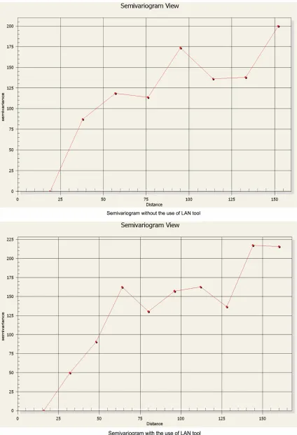
Kriging is based on the assumption that for a given point data set those that are close to each other are corre-lated whereas those at a further distance are statistically independent [23]. Its basic idea is equivalent to inverse distance weighted interpolation but instead of using weights based on an arbitrary function of distance in or-der to compute an interpolated point, the weights used in kriging are based on the model variogram. The model variogram is derived after constructing the experimental variogram from the point data set to be interpolated, like the one presented in Figure 7.

The experimental variogram is calculated by deter-mining the variance of each data point in the data set with respect to all other data points and by plotting the variances (or semivariances) versus distance between points. The model variogram is then defined as a simple mathematical function that best fits the experimental variogram. As it can be seen on Figure 7, for small separating distances the variance of the variable to be interpolated is small whereas after a certain distance the variance becomes random. The model variogram is used to compute the weights used in kriging in order to evalu-ate an interpolevalu-ated value F of the variable f based on the

following equation:

 

i i i 1

F x, y w f







where n in the number of points in the set, fi are the val-ues of those points and wi are the weights assigned to each data point. In that way, if a new interpolated value P it to be calculated from three neighboring points P1, P2, P3 then w1, w2 and w3 have to be determined solving a system of 3 equations based on the values of the model variogram evaluated at a distance equal to the distance between points i and j.

Figure 7. Comparison of semi variograms produced with and without the use of LAN tool, to the semi variogram with meas-red altitude data.

3. Results and Discussion

3.1. Application to TA1

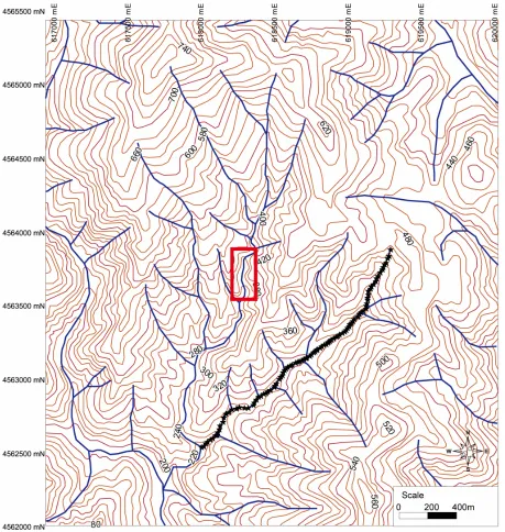
Figure 8 shows the altitude contours and the drainage

network of TA1. In order to test the efficiency of the proposed methodology, DEM construction in TA1 was achieved with and without the use of LAN tool. The kriging interpolation technique was used in either case, as mentioned previously. The acquired results were com- pared to measured values of altitude performed using a

Trimble GPS Total Station R4.

Two independent tests were then performed; the first one compares the semi variograms produced with 50 measured altitude points, to those produced with the data points before and after the use of LAN tool in a small portion of TA1 highlighted as a red rectangle on Figure 8. In each case the lag distance used was the mean dis-tance between data points. Figure 7 shows the semi variograms produced using only measured altitude points and those produced with and without the use of LAN tool.

Figure 8. Map of TA1. Red rectangle highlights the area where semi variograms with and without the use of LAN tool, were compared to the semi variogram with measured data. Black spots indicate locations where altitude measurements on a main

It can be seen that all three semi variograms present the same trend but the semi variograms of the measured points and that using points produced with LAN tool are almost identical.

The second test compares the altitude values produced with and without the application of LAN tool to meas-ured altitude values on 100 randomly sampled data po- ints located on one of the main branches of the drainage network of TA1 shown as black points on Figure 8. Fig-

ure 9(a) shows the river profiles produced with the

measured altitude points and with and without the use of LAN tool. As it can be seen the profile produced using LAN tool is much closer to the measured one.

The mean absolute error (MAE) was calculated for the two profiles produced with and without the use of LAN tool, based on the following formula:

N t t t 1

1 _ˆ

MAE Z Z

N 





Zt being the interpolated altitude values, t the meas-ured altitude values and N the number of points, which in our case is 100.

ˆ Z

The MAE for the profiles produced with and without the use of LAN tool is 0.58 m and 2.39 m respectively.

Figures 9(b) and (c) present the DEMs produced with-out and with the use of LAN tool, respectively. From a

(a)

(b) (c)

Figure 9. Cross sectional plot of a river branch produced with and without the use of LAN tool and with measured altitude alues.

first point of view the DEMs produced using either method are very similar, but based on the comparison to the measured values, the LAN tool improved the pro-duced DEM.

3.2. Application to TA2

In contrast to TA1, which is almost unaffected by human intervention, TA2 has undergone changes of the natural route of the drainage network, changing the main course of Vosvozis river and constructing irrigation and drain-age channels. Additionally, Ismarida lake which is an important ecosystem, has decreased seriously in the last decade due to excess pumping. Thus, the topography of the area is also altered, which is not represented in the conventional maps that cannot be updated continuously. The main problem that arose is that when the DEM of TA2 was constructed, using topographic data from those conventional maps, the drainage network that was de-lineated using hydrologic models did not correspond to the existing network. Moreover, in plain areas, even in cases where no major human interventions have taken place, altitude contours are sparse, thus even the small errors associated with the interpolation technique may result in depressions that hinder flow or a drainage pat-tern which deviates considerably from the existing one. In those cases, the use of LAN tool proves to be quite useful for DEM correction. As LAN tool requires the river network to be provided, an ASTER image of the study area acquired in August 2009 was used for the de-lineation of the river network (Figure 10).

Figure 10. Aster image acquired on August 2009, showing the river network of TA2.

Topographic data were digitized using conventional topographic maps of the Hellenic Military Geographical Service of scale 1:5000. Kriging interpolation was used to create a DEM, with and without the use of LAN tool. The produced DEMs were introduced to one of the most popular hydrologic models, i.e. Soil and Water Assess-ment Tool (SWAT) [25], in order to delineate automati-cally the drainage network. The results were compared to the existing drainage network. Figure 10 shows the drainage network delineated from the ASTER image.

Figure 11(a) shows the drainage network produced by

automatic delineation using the DEM without the use of LAN tool (Figure 11(b)).

Figure 12(a) shows the drainage network produced by

automatic delineation using the DEM with the use of LAN tool shown on Figure 12(b). Comparison of the produced results shows that the river network delineated based on the DEM with the use of LAN tool is much closer to the real one. Additionally, one can easily dis-tinguish the artificial irrigation pond shown on the north east of Figure 12(b), which is incorporated in the DEM using LAN tool. Thus LAN tool proved to be quite effec-tive in TA2.

At this point the findings of the research conducted by Chaplot et al. [12] should be mentioned. They found that irrespective of the surface area, landscape morphology and sampling density, few differences existed between the employed interpolation techniques if the sampling density was high. At lower sampling densities, in con-trast, the performance of the techniques tended to vary. Within this context the usefulness of LAN tool is unam-biguous at it increases sampling density in specified lo-cations where most of the DEM inaccuracies tend to exist. Besides the fact that kriging was used for demonstration purposes, the same improved results on the DEM are expected with all other interpolation techniques, as LAN tool does not alter the interpolation itself, but it provides a higher point data density in areas of interest.

4. Conclusions

(a) (b)

Figure 11. (a) River network produced with automatic delineation using SWAT model using DEM without the use of LAN tool; (b) DEM produced without the use of LAN tool.

(a) (b)

Figure 12. River network produced with automatic delineation using SWAT model using DEM with the use of LAN tool; (b) DEM produced with the use of LAN tool.

achieved, as indicated by the minimization of MAE. In the second case, i.e. TA2, where serious interven-tions on the drainage network had taken place, the im-provement using LAN tool was obvious, as the produced

DEM represented accurately the current pattern of the drainage network.

attribute network. Analogous applications may well be developed using LAN tool with other line attribute net-works, like roads or any other linear feature.

5. Acknowledgements

The field measurements conducted in the present work were part of the project: “Water resources management in Eastern Macedonia and Thrace” funded by the Tech-nical Chamber of Greece (project code: 2237 Democritus University of Thrace).

REFERENCES

[1] C. Legleiter and P. Kyriakidis, “Spatial Prediction of Ri- ver Channel Topography by Kriging,” Earth Surface Pro- cesses and Landforms, Vol. 33, No. 6, 2008, pp.841-867. doi:10.1002/esp.1579

[2] V. Chaplot, “Impact of DEM Mesh Size and Soil Map Scale on SWAT Runoff, Sediment, and NO3-N Loads Pre-

dictions,” Journal of Hydrology, Vol. 312, No. 1-4, 2005, pp. 207-222.

[3] L. Kalin, R. S. Govindarajua and M. M. Hantush, “Effect of Geomorphologic Resolution on Modeling of Runoff Hydrograph and Sedimentograph over Small Watersheds,”

Journal of Hydrology, Vol. 276, No. 1-4, 2003, pp. 89- 111. doi:10.1016/S0022-1694(03)00072-6

[4] A. R. Darnell, A. A. Lovett, J. Barclay and R. A. Herd, “An Application Driven Approach to Terrain Model Construc- tion,” International Journal of Geographical Information Science,Vol. 24, No. 8, 2010, pp. 1171-1191.

doi:10.1080/13658810903318889

[5] J. Kiesel, N. Fohrer, B. Schmalz and M. J. White, “In- corporating Landscape Depressions and Tile Drainages of a Northern German Lowland Catchment into a Semi-Dis- tributed Model,” Hydrological Processes, Vol. 24, No. 11, 2010, pp. 1472-1486. doi:10.1002/hyp.7607

[6] H. Achour, N. Rebai, J. Van Den Driessche and S. Boua- ziz, “Modelling Uncertainty of Stream Networks Derived from Elevation Data Using Two Free Softwares: R and SAGA,” Journal of Geographic Information System, Vol. 4, No. 2, 2012, pp. 153-160. doi:10.4236/jgis.2012.42020 [7] D. Weber and E. Englund, “Evaluation and Comparison

of Spatial Interpolators,” Mathematical Geology, Vol. 24, No. 4, 1992, pp. 381-391. doi:10.1007/BF00891270

[8] D. Weber and E. Englund, “Evaluation and Comparison of Spatial Interpolators II,” Mathematical Geology, Vol. 26, No. 5, 1994, pp. 589-603. doi:10.1007/BF02089243

[9] A. Carrara, G. Bitelli and R. Carla, “Comparison of Tech- niques for Generating Digital Terrain Models from Con- tour Lines,” International Journal of Geographical In- formation Science, Vol. 11, No. 5, 1997, pp. 451-473. doi:10.1080/136588197242257

[10] S. M. Robeson, “Spherical Methods for Spatial Interpola- tion: Review and Evaluation,” Cartography and Geogra- phic Information Systems, Vol. 24, No. 1, 1997, pp. 3-20. doi:10.1559/152304097782438746

[11] F. J. Aguilar, F. Agüera, M. A. Aguilar and F. Carvajal,

“Effects of Terrain Morphology, Sampling Density, and Interpolation Methods on Grid DEM Accuracy,” Photo- grammetric Engineering and Remote Sensing, Vol. 71, No. 7, 2005, pp. 805-816.

[12] V. Chaplot, F. Darboux, H. Bourennane, S. Leguédois, N. Silvera and K. Phachomphon, “Accuracy of Interpolation Techniques for the Derivation of Digital Elevation Mod- els in Relation to Landform Types and Data Density,”

Geomorphology, Vol. 77, No. 1-2, 2006, pp. 126-141. doi:10.1016/j.geomorph.2005.12.010

[13] S. J. Buckley and H. L. Mitchell, “Integration, Validation and Point Spacing Optimization of Digital Elevation Mo- dels,” The Photogrammetric Record, Vol. 19, No. 108, 2004, pp. 277-295.

doi:10.1111/j.0031-868X.2004.00287.x

[14] M. Karkee, B. L. Steward and S. A. Aziz, “Improving Quality of Public Domain Digital Elevation Models through Data Fusion,” Biosystems Engineering, Vol. 101, No. 3, 2008, pp. 293 -305.

doi:10.1016/j.biosystemseng.2008.09.010

[15] W. Z. Shi and Y. Tian, “A Hybrid Interpolation Method for the Refinement of a Regular Grid Digital Elevation Model,” International Journal of Geographical Informa- tion Science, Vol. 20, No. 1, 2006, pp. 53-67.

doi:10.1080/13658810500286943

[16] O. Bonin and D. Rousseaux, “Digital Terrain Model Com- putation from Contour Lines: How to Derive Quality In- formation from Artifact Analysis,” GeoInformatica, Vol. 9, No. 10, 2005, pp. 253-268.

doi:10.1007/s10707-005-1284-2

[17] Y. Chen, J. P. Wilson, Q. Zhu and Q. Zhou, “Comparison of Drainage-Constrained Methods for DEM Generaliza- tion,” Computers and Geosciences, Vol. 48, 2012, pp. 41- 49. doi:10.1016/j.cageo.2012.05.002

[18] W. Saunders, “Preparation of DEMs for Use in Environ- mental Modelling Analysis,” In: D. Maidment and D. Djokic, Eds., Hydrologic and Hydraulic Modelling Sup- port with Geographic Information Systems,Environmen- tal Systems Research Institute Inc., Redlands, 2000, pp. 29-51.

[19] J. N. Callow, K. P. Van Niel and G. S. Boggs, “How Does Modifying a DEM to Reflect Known Hydrology Affect Subsequent Terrain Analysis?” Journal of Hydrology, Vol. 332, No. 1-2, 2007, pp. 30-39.

doi:10.1016/j.jhydrol.2006.06.020

[20] M. F. Hutchinson, “A New Procedure for Gridding Ele- vation and Stream Line Data with Automatic Removal of Spurious Pits,” Journal of Hydrology, Vol. 106, No. 3-4, 1989, pp. 211-232. doi:10.1016/0022-1694(89)90073-5

[21] Q. Zhou and Y. Chen, “Generalization of DEM for Ter- rain Analysis Using a Compound Method,” ISPRS Jour- nal of Photogrammetry and Remote Sensing, Vol. 66, No. 1, 2011, pp. 38-45. doi:10.1016/j.isprsjprs.2010.08.005

[22] D. Souvaine, “Line Segment Intersection Using a Sweep Line Algorithm,” Tufts University, 2005.

http://www.cs.tufts.edu/comp/163/notes05/seg_intersectio n_handout.pdf

[24] G. S. Carter and U. Shankar, “Creating Rectangular Ba- thymetry Grids for Environmental Numerical Modelling of Gravel-Bed Rivers,” Applied Mathematical Modelling, Vol. 21, No. 11, 1997, pp. 699-708.

doi:10.1016/S0307-904X(97)00094-2