The Effect of Pension on the Optimized
Life Expectancy and Lifetime Utility
Level
Shin, Inyong
Asia University
September 2012
Online at
https://mpra.ub.uni-muenchen.de/41375/
and Lifetime Utility Level
Inyong Shin∗
Abstract
In this paper, we analyze the effect of a pension system on the life expectancy and the
lifetime utility level using an optimal dynamic problem of individuals who live in continuous
and finite time. Our model yields a number of intriguing results: 1) Life expectancy is not
always proportional to lifetime utility. 2) The pension system can make life expectancy longer
or shorter. 3) It is not always true that the pension system improves the lifetime utility level.
JEL Classification Codes: C61, H55, I31
Keywords: Pension system, Optimized life expectancy, Lifetime utility level, Health invest-ments
1
Introduction
According to an anecdote in Europe, as soon as a pension system was introduced, the number of
people who jog in the park for their health increased. Believe it or not. Anyway, under pension
system, it looks like a good deal, if we live long enough. This paper analyzes the effect of a pension
system on the life expectancy and the lifetime utility level. Bloom et al. (2007) and Dushi et
al. (2010), etc. examine the effect of improvements in health or life expectancy on social security
system, however, we focus on the effect on the opposite direction.1
A vest amount of emprical and theoretical researches about the pension system has been
accumulated. Many previous researches analyze economic welfare using overlapping generation
∗Department of Economics, Asia University,
5-24-10 Sakai Musashino Tokyo 180-8629 Japan, Tel.: +81-422-36-5259,
Fax: +81-422-36-4042,
e-mail addredss: [email protected]
models. The main results of some previous studies on pension system and economic welfare can be
summarized as follows: under a fully funded system, the economic welfare is not affected, however,
under a pay-as-you-go pension system, depending on the economic situations and generations, the
economic welfare might be both improved and worsened. The public pension system as a
risk-hedging device can increase welfare by providing a certainty in the imperfect market. (Shiller,
1999, Krueger and Kubler, 2002, S´anchez-Marcos and S´anchez-Martin, 2006, Bohn, 2009, etc.)
Meanwhile, the public pension system crowds out the private savings. It can have a negative
effect on capital accumulation and can retard growth. (Cutler and Gruber, 1996, Feldstein and
Liebman, 2002, Zhang and Zhang, 2004, etc.) The overall welfare impact depends on the balance
between the insurance effect and the crowding-out effect.
We use the optimal dynamic problem of individuals who live in continuous time, not discrete
time like the overlapping generation models used in the presvious studies. (e.g. S´anchez-Marcos
and S´anchez-Martin, 2006) This is one of the difference of our model from the previous models. In
lifetime uncertainty models, e.g. Pecchenino and Pollard (1997), Chakraborty (2004), Momota,
et al (2005), etc., we assume that it is possible to extend life span by the effort of an individual
through health investments.2 For examples, eating good food, taking some nutritional supple-ments, getting in shape by going to the gym, investing in development of medical technology, etc.
Longevity will arise due to the given examples on health investments. An individual distributes
his budget to his basic needs and to his health investments to maximize his lifetime utility. We
consider that individual’s longevity is based from the result of individual’s utility maximization
problem. We investigate how the optimized life span and the lifetime utility level can be changed
by a pension system.
Our model yields two impotant results: i) Life expectancy is not always proportional to lifetime
utility level. ii) Pension system can make the life span longer or shorter. The life span depends on
the type of pension system. From the combination of the results i) and ii), it is possible that 1)
pension system makes the life span longer and increases the utility level. 2) pension system makes
the life span longer, however decreases the utility level. 3) pension system makes the life span
shorter and decreases the utility level. Case 1 is preferable. but Case 2 and 3 are not preferable
cases, but could possibly happen.
This paper is organized as follows: Section 2 presents the model and drives the benchmark
outcomes. In section 3, we introduce the pension system to the benchmark. Section 4 solves the
models numerically and analyzes the results and concludes. And finally, we include an Appendix.
2
The benchmark Model
2.1 Setting
We consider an individual’s utility maximization problem under the finite period. He can live up
to T years old and dies at the age of T. An individual maximizes his lifetime utility which is
affected by consumption. The instantaneous utility function is specified in log form as follows:
u(c) = lnc (1)
where c is a consumption. We think that it is possible to extend the life span by the efforts of
the individual. We assume that there is a linear relationship between health investment and life
span as follows
T =a+bz, (a >0, b >0) (2)
where T and z are life span and health investment, respectively. And a and b are positive
constants. We assume that the health investments do not affect the utility directly.3 We also assume that the interest earning is the only source of income of the individual. And to simplify,
a small country is assumed, then the interest rate is constant at all period. Let us denote the
individual’s asset asx, then his budget constraint is written as:
˙
x=rx−c−z (3)
wherer is an interest rate.
An individual’s utility maximization problem can be written as follows:
max
c(t),T
∫ T
0
e−ρtlnc(t) dt, (0< ρ <1)
s.t x˙(t) =rx(t)−c(t)−z
(4)
3We can divide the consumption
cinto two categories. These are the general consumptioncGand the
consump-tion for health improvementcH. The effect of the lattercH on the utility of individual is unclear whether positive
whereρis a discount rate. We assumer≥ρ.4 For simplification, we assume thatzhas a constant
value from initial period untilT period and thatz is decided at the initial period. In unrealistic
assumption, we assume that as an individual is born, he decides how much he invests for his
health and how long he lives under a social environment.
2.2 Solving the Model
The maximization problem is solved in two stages. At the first stage, we do not consider the Eq.
(2). Maximize over c and x for any given T and z, and then the objective function maximized
with respect to c and x could be described as a function of T and z. At the second stage, we
consider the Eq. (2). Maximize over T and z taking into accountcobtained in the first stage.
2.2.1 The First Stage
We use the Hamiltonian method to solve the maximization problem. The Hamiltonian is written
as follows:
H = lnc+λ(rx−c−z) (5)
By differentiating Eq. (5) with respect toc and x, we can get Eq. (6) and Eq. (7).
∂H ∂c =
1
c −λ= 0 ⇒ c=λ
−1, (6)
∂H
∂x =ρλ−λ˙ =λr ⇒ ˙ λ
λ =ρ−r. (7)
We integrate Eq. (7) to timet, then we get
lnλ= (ρ−r)t+k (8)
wherek is a constant of integration. Taking exponential both sides of Eq. (8), then we can get
λ=C1e(ρ−r)t (9)
whereC1 =ek. Substituting Eqs. (6) and (9) into Eq. (3), we obtain the following
˙
x−rx+z=−C−1
1 e−ρtert. (10)
4If
r=ρ, there is no transitional path, because the jump from the initial state upto the terminal state occurs. Ifr < ρ, there is an overshooting, the economy turns back to the terminal state and has a negative growth rate.
This differential equation is solved as folllow
x= 1 C1
(e−ρt−1
ρ
)
ert+C2ert+z
r (11)
where C2 is a constant. See Appendix for the detailed calculation. C1 and C2 can be obtained
from substituting the initial condition and transversality condition. Let us x(0) = x0, then we
getC2 as follows
C2=x0−z
r. (12)
To maximize his utility, when dying, he uses up all his asset and leave nothing. In other words,
x(T) = 0. We getC1 as follows
C1 =
1 ρ
1−e−ρT
x0−(1−e−rT)zr
. (13)
Substituting Eqs. (12) and (13) into Eq. (11), we obtain the following
x(t) = x0−(1−e
−rT)z
r
1−e−ρT (e
−ρt−1)ert+ (x
0−
z r)e
rt+z
r. (14)
Substituting Eq. (9) into Eq. (6), we can get
c(t) =ρx0−(1−e
−rT)z
r
1−e−ρT e
(r−ρ)t. (15)
Eqs. (14) and (15) are the optmal paths of x and c, repectively by regarding the variableT and
z as fixed.
2.2.2 The Second Stage
In the second stage, to maximize his lifetime utility, the individual chooses his optimal T with
considering Eq. (2). We can rewrite the utility maximization problem as follows:
max
T
∫ T
0
e−ρtln(ρx0−(1−e −rT)z
r
1−e−ρT e
(r−ρ)t) dt
s.t T =a+bz
(16)
We solve the integral in Eq. (16), then we can induce Eq. (17)
∫ T
0
e−ρtln(ρx0−(1−e −rT)z
r
1−e−ρT e
(r−ρ)t)dt
=−ln(ρx0−(1−e
−rT)z
r
1−e−ρT
)(e−ρT −1
ρ
)
−(r−ρ)((ρT + 1)e
−ρT −1
ρ2
)
(17)
See Appendix for the detailed calculation. Substituting Eq. (2) into Eq. (17), Eq. (16) can be
rewritten as Eq. (18) which has no integral and has only one control variableT. Eq. (18) is just
a static maximization problem, not a dynamic one.
max
T ln
(
ρx0−(1−e
−rT)T−a
rb
1−e−ρT
)(1−e−ρT
ρ
)
+ (r−ρ)(1−(ρT + 1)e−
ρT
ρ2
)
We take the derivative of Eq. (18) with respect to T and set the first derivative to zero.
e−ρTln(ρx0−(1−e
−rT)T−a
br
1−e−ρT
)
−1−e−
ρT
ρb
e−rT(T−a) + (1−e−rT)1
r
x0−(1−e−rT)Tbr−a
−e−ρT+ (r−ρ)T e−ρT = 0
(19)
Eq. (19) is an implicit function asf(x0, T|a, b, r, ρ) = 0 which is highly non linear and difficult to
solve analytically.
3
Pension System
We introduce a pension system into the benchmark model. He pays a pensionpfrom 0 tosperiod,
gets a pension q after s period. Government decidesp,q and swhich are constants as given to
individuals. This pension system plays as a compulsory saving for individuals. For simplification,
we do not consider the balanced budget of the government for the pension system. It can be a
fully funded system or a pay-as-you-go pension system, because we do not need to consider where
the financial resources of pension come from, under the situation where there is no need for the
balanced budget.
We shall call the period from 0 to s period as young period and aftersperiod as old period.
His budget constraint Eq. (3) is changed to Eq. (20).
˙ x=
rx−c−z−p, if 0≤t≤s rx−c−z+q, if s < t≤T.
(20)
The way to solve the model with this pension system is similar to that of the benchmark model
even though we have to divide it into young period and old period. Eq. (11) is changed as follow
x= 1 CY 1 (
e−ρt−1
ρ
)
ert+C2Yert+ z+rp, if 0≤t≤s
1
CO
1
(
e−ρt −1
ρ
)
ert+CO
2 ert+z−rq, if s < t≤T.
(21)
where, C1Y,C2Y,C1O andC2O are constants of integration which are as follows:
C1Y = 1 ρ
1−e−ρs
x0−(1−e−rs)z+rp −x(s)e−rs
(22)
C2Y =x0−
z+p
r (23)
C1O= 1 ρ
(e−ρT −e−ρs)ers z−q
r (1−er(s−T))−x(s)
C2O=
z−q
r (1−e
r(s−T))−x(s)
(e−ρT −e−ρs)ers (1−e
−ρT)− z−q
r e
−rT (25)
where, x(s) is interpreted as both the terminal value of young period and the initial value of old
period at the same time. By the same way as the previous, Eq. (15) is changed as follows
c(t) =
1
C1Ye
(r−ρ)t, if 0≤t≤s
1
CO
1
e(r−ρ)t, if s < t≤T.
(26)
Substituting Eq. (26) into the utility function, we obtain the following
∫ s
0
e−ρtln( 1
C1Y e
(r−ρ)t) dt+
∫ T
s
e−ρtln( 1
C1Oe
(r−ρ)t)dt (27)
We integrate Eq. (27) to timet, then we get
ln( 1 CY
1
)1−e−ρs
ρ + ln
( 1
CO
1
)e−ρs−e−ρT
ρ −(r−ρ)
((ρT + 1)e−ρT −1
ρ2
)
. (28)
There are z’s in CY
1 ,C2Y,C1O and C2O. We substitute z = T−ba intoC1Y,C2Y,C1O and C2O, then,
the original dynamic optimization problem with the pension system is nothing less than the static
optimization problem with respect toT and x(s) as seen in Eq. (29). In other words, all he has
to do is just to decide his own life expectancy and the initial asset at the old period.
max
T,x(s)U
(
T, x(s))
= ln( 1 CY
1
(
T, x(s))
)1−e−ρs
ρ + ln
( 1
CO
1
(
T, x(s))
)e−ρs−e−ρT
ρ
−(r−ρ)((ρT + 1)e−
ρT −1
ρ2
)
(29)
4
Results and Conclusion
Taking the derivative of Eq. (29) with respect toT andx(s), and setting each first derivatives to
zero, and solving the system of equations, we could obtain the optimal T∗ and x(s)∗. Since the
profit function of Eq. (29) is highly nonlinear, however, it is very difficult to get an exact analytical
solution for this problem. The alternative option is to provide the solutions numerically. The
suitable parameter values are used for the calculation, though they are arbitrary. The parameter
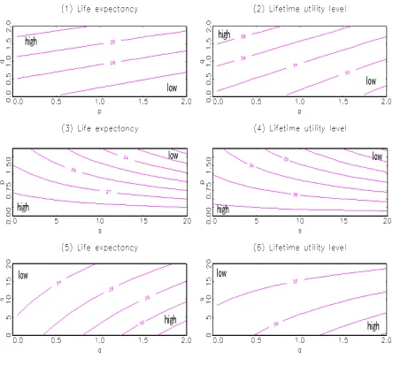
values that we used to calculate are the following: a= 20, b= 10,x0 = 100,ρ = 0.01, r = 0.02.
To show the effect ofp,q andson life expectancy and lifetime utility,pandq are controlled from
0.0 to 2.0, andsis controlled from 0.0 to 20.
Each panel in Figure 1 shows the results as the coutour lines. Figure 1(1) and 1(2) show the
Figure 1: Life expectancy and lifetime utility level
whilepandq are changed. In Figure 1(1) and 1(2), the values on the left-upper side are high and
the values on the right-lower side are low. Under fixed s, when p is small and q is big, the life
expectancy is longer and the lifetime utility level is higher. Figure 1(3) and 1(4) show the results
of the life expectancy and the lifetime utility level, respectively, whenq is fixed at 1.0 whilepand
sare changed. In Figure 1(3) and 1(4), the values on the left-lower side are high and the values
on the right-upper side are low. Under fixed q, whenp is small andsis short, the life expectancy
is longer and the lifetime utility level is higher. Figure 1(5) and 1(6) show the results of the life
expectancy and the lifetime utility level, respectively, when p is fixed at 1.0 while q and s are
changed. In Figure 1(5) and 1(6), the values on the right-lower side are high and the values on
longer and the lifetime utility level is higher.
To summarize these results, when pis small, whenq is big, and whensis short, that is, when
an individual pays a small amount of money for a short period of time and gets a big amount
of money from his pension, the life expectancy is longer and the lifetime utility level is higher.
These results accord with intuition.
21 22 23 24 25 26 27 28 29 30 31 32 33
27.5
30.0
32.5
35.0
37.5
40.0
42.5
Life expectancy
Lifetime utility level
I
II
III
IV
[image:10.595.108.488.206.460.2]A
Figure 2: Comparison of the results with and without the pension system
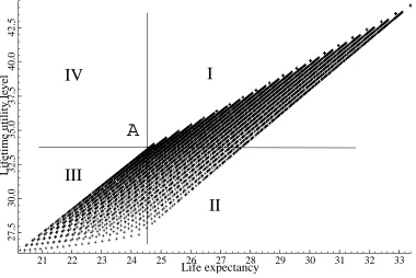
Figure 2 plots the relationship between the life expectancy and the lifetime utility level. The
horizontal line and the vertical line present the life expectancy and the lifetime utility level,
respectively.5 The +’s in Figure 2 are the corresponding values of the life expectancy in Figure 1(1), 1(3) and 1(5), and the lifetime utility level in Figure 1(2), 1(4) and 1(6). And point A
(24.556, 33.742) shows the pair of the life expectancy and the lifetime utility level obtained from
the benchmark model. All of these +’s except point Ashow the pairs when the pension system
exists in some way or another. We draw a vertical and horizontal line from pointAand divide the
plain into 4 areas. In area I, the life expectancy is longer and the lifetime utility level is higher
compared to pointA. In area II, the life expectancy is longer but the lifetime utility level is lower
compared to point A. In area III, the life expectancy is shorter and the lifetime utility level is
lower compared to pointA. There is no pair in area IV.
The life expectancy is not always proportional to the lifetime utility level. Comparing with a
’+’ in area II and point A, even though the life expectancy is longer, the lifetime utility level is
lower. And the pension system can make life expectancy longer or shorter and can make lifetime
utility level higher or lower. If we get big amount of pension in the future, the life expectancy
can be extended and the lifetime utility can go up. It is the most preferable, however, in today’s
reality, the pension system cannot avoid the problem of financial resources.
The pension system could also lead to some kind of infirmity as follows: 1) Even though the
life expectancy is extended, the lifetime utility level goes down. By that, an individual is forced to
pay the pension during his young period, the pension system leads to less personal consumption
in his young period. Even though he tries to prolong his life for a long time to get his money back
which he paid mandatorily, his lifetime utility level can go down compared to a case of no pension
system. 2) The life expectancy is decreased, moreover, the lifetime utility level goes down. This
is the worst scenario. An individual can choose a short life to refuse to pay the pension until such
period sand to increase his consumption in his young period.6
It is not always true that the pension system improves the lifetime utility level as shown in
area II and III in Figure 2. Not only the government has to exert effort to avoid infirmities as
stated above, but the government also has to reconsider about the raison d’etre (the reason for
existance) of the compulsory pension system.
Appendix
Derivation of Eq. (11)
Let us put B =−C−1
1 . Multipling both sides of Eq. (10) bye−rt and integrating to time t, we
get the following
( ˙x−rx+z)e−rt=Be−ρt
xe−rt−z
re
−rt+D
1=−B
e−ρt
ρ +D2
(A1)
whereD1 and D2 are constants of integration. Eq. (A1) can be arranged as follows
xe−rt− z
re
−rt=−Be−
ρt
ρ +B 1 ρ +C2
(
x−z
r
)
e−rt=−B(e −ρt−1
ρ
) +C2
(A2)
whereC2=D2−D1−Bρ1. Multipling both sides of Eq. (A2) bye−rt and substitutigB=−C1−1
into Eq. (A2), Eq. (A2) can be arranged as Eq. (11).
Derivation of Eq. (17)
Let us putA= ln(ρx0−(1−e−
rT)z r
1−e−ρT
) .
∫ T
0
e−ρtln(ρx0−(1−e −rT)z
r
1−e−ρT e
(r−ρ)t) dt =
∫ T
0
[
Ae−ρt+ (r−ρ)te−ρt]
dt
=A
∫ T
0
e−ρt dt+ (r−ρ)
∫ T
0
te−ρt dt =A[−e−ρt
ρ
]T
0 −(r−ρ)
[(ρt+ 1)e−ρt
ρ2
]T
0
=−A(e
−ρT −1
ρ
)
−(r−ρ)((ρT+ 1)e
−ρT −1
ρ2
)
(A3)
Substitutig A= ln(ρx0−(1−e−rT)
z r
1−e−ρT )
into Eq. (A3), Eq. (A3) can be arranged as Eq. (17).
References
[1] Acemoglu, D., and Johnson, S., 2007. Disease and Development: The Effect of Life
Ex-pectancy on Economic Growth,Journal of Political Economy, Vol.115(6), pp.925-985.
[2] Bloom, D., Canning, D., Mansfield, R., and Moore, M. j., 2007. Demographic change, social
security systems, and savings,Journal of Monetary Economics, vol. 54(1), pp.92-114.
[3] Bohn, H., 2009. Intergenerational risk sharing and fiscal policy, Journal of Monetary
Eco-nomics, Vol.56(6), pp.805-816.
[4] Chakraborty, S., 2004. Endogenous lifetime and economic growth,Journal of Economic
The-ory, Vol.116, pp.119-137.
[5] Cutler, D. M., and Gruber, J., 1996. Does Public Insurance Crowd Out Private Insurance?,
[6] Dushi, I., Friedberg, L., and Webb, T., 2010. The impact of aggregate mortality risk on
defined benefit pension plans,Journal of Pension Economics and Finance, Vol.9(4), pp.481-503.
[7] Feldstein, M. S., and Liebman, J. B., 2002. The Distributional Aspects of Social Security
and Social Security Reform, NBER Chapters, pp.263-326. National Bureau of Economic
Research, Inc.
[8] Krueger, D., and Kubler, F., 2002. Intergenerational Risk Sharing via Social Security when
Markets are Incomplete,American Economic Review, Vol.92(2), pp.407-410.
[9] Momota, A., Tabata, K., and Futagami, K., 2005. Infectious disease and preventive behavior
in an overlapping generations model,Journal of Economic Dynamics and Control, Vol.29(10), pp.1673-1700.
[10] Pecchenino, R. A., and Pollard, P. S., 1997. The effects of annuities, bequests, and aging in an
overlapping generations model of endogenous growth,Economic Journal, Vol.107, pp.26-46.
[11] S´anchez-Marcos, V., and S´anchez-Martin, A. R., 2006. Can social security be welfare
improv-ing when there is demographic uncertainty?, Journal of Economic Dynamics and Control, Vol.30(9-10), pp.1615-1646.
[12] Shiller, R., 1999. Social Security and Institutions for Intergenerational, Intragenerational
and International Risk Sharing, Carnegie-Rochester Conference Series on Public Policy, Vol.50(1), pp.165-204.
[13] Weil, D. N., 2007. Accounting for the Effect of Health on Economic Growth, Quarterly
Journal of Economics, Vol.122(3), pp.1265-1306.
[14] Zhang, J. and Zhang, J., 2004. How Does Social Security Affect Economic Growth? Evidence
from Cross-Country Data,Journal of Population Economics, Vol.17(3), pp.473-500.
[15] Zhang, J., Zhang, J., and Lee, R., 2001. Mortality decline and long-run economic growth,