Accounting for non annuitization

Munich Personal RePEc Archive

Accounting for non-annuitization

Pashchenko, Svetlana

Uppsala University

19 November 2012

Online at

https://mpra.ub.uni-muenchen.de/42792/

Accounting for non-annuitization

∗

Svetlana Pashchenko

Uppsala University

November 19, 2012

Abstract

Why don’t people buy annuities? Several explanations have been provided by the previous literature: large fraction of preannuitized wealth in retirees’ portfo-lios; adverse selection; bequest motives; and medical expense uncertainty. This paper uses a quantitative model to assess the importance of these impediments to annuitization and also studies three newer explanations: government safety net in terms of means-tested transfers; illiquidity of housing wealth; and restrictions on minimum amount of investment in annuities. This paper shows that quantita-tively four explanations play a big role in reducing annuity demand: preannuitized wealth, minimum annuity purchase requirement, illiquidity of housing wealth, and bequest motives. The annuity purchase involves big upfront investment, especially if there is a minimum purchase restriction. This is binding for many, especially if housing is illiquid and part of wealth is preannuitized. While bequest motives significantly reduce the overall annuity demand, the model with a strong bequest motive cannot match the empirical fact that high-income people have the highest demand for annuities.

Keywords: annuity puzzle, longevity insurance, adverse selection

JEL Classification Codes: D91, G11, G22

∗_{I am grateful to Mariacristina De Nardi, Leora Friedberg, Toshihiko Mukoyama, and Eric Young for}

their help and support. I also thank Gadi Barlevy, Marco Bassetto, Emily Blanchard, Jeffrey Brown, Jeffrey Campbell, Thomas Davidoff, Eric French, John Jones, Alejandro Justiniano, Lee Lockwood, Ponpoje Porapakkarm, Richard Rosen, Dan Silverman, three anonymous referees and seminar partici-pants at the Federal Reserve Bank of Chicago, Netspar Pension Workshop, Midwest Macro Meeting in East Lansing, SED in Montreal, Retirement Research Consortium, IFID and NTA annual meetings, and QSPS Summer Workshop for their comments and suggestions. Financial support from the Center of Retirement Research at Boston College, Bankard Fund for Political Economy, Committee on the Status of Women in the Economics Profession and the hospitality of the Federal Reserve Bank of Chicago are gratefully acknowledged. All errors remain my own.

1

Introduction

A well-known prediction of the standard life-cycle model is that in the presence of lifespan uncertainty, people should invest in nothing but annuities (Yaari, 1965). In practice few people buy annuities. This empirical fact is called the ”annuity puzzle”. The literature seeking to explain this puzzle has mainly attributed the lack of interest in annuities to the following four factors: a substantial fraction of preannuitized wealth in retirees’ portfolios, actuarially unfair prices, bequest motives, and uncertain health expenses. It is still an open question, however, what is the relative quantitative impor-tance of different explanations for the annuity puzzle. The goal of this paper is therefore to provide a quantitative analysis of people’s decisions to buy annuities in a model that nests all major impediments to annuitization.

I develop a quantitative model of saving after retirement in which individuals face lifespan uncertainties that create a demand for longevity insurance. At the same time the available annuities are illiquid, i.e., they entitle a person to a constant stream of income that cannot be converted back to liquid wealth. The other key features of the model are uncertain medical expenses, bequest motives, preannuitized wealth, and the government-provided minimum consumption level. Augmented in this way, the life-cycle model allows for states, when it is not optimal for an individual to lock his wealth in a constant stream of income.

Another important feature of the model is that annuity prices are determined in equilibrium. When modeling the annuity market I compare two information structures. In the first, the insurer and the annuity buyer have the same information about the mortality of the latter. In the second, there is asymmetric information, and the insurer can only observe the age of the annuity buyer. The latter scenario creates an environment for adverse selection which is intensified by the negative correlation between wealth and mortality. This happens because retirees with low mortality buy more annuities because they not only expect to live longer but are also wealthier.

The main quantitative exercise of this paper consists of comparing annuity market participation rates between the models that incorporate different impediments to annu-itization. I study seven explanations for the annuity puzzle: four traditional ones and three factors that have been studied much less. The latter include government provided social assistance, difficulties with annuitizing housing wealth, and a minimum purchase requirement set by insurance companies.

The consumption minimum floor, among other things, provides financial support for people if they outlive their assets and thus offers some longevity insurance. This public longevity insurance may partially substitute for a private annuity, at least for low-income retirees.

long period of time and, as such, involve a big upfront investment. When it comes to buy-ing an annuity, liquidity constraints may therefore become an issue because, first, housbuy-ing wealth may not be easily annuitized and, second, insurance firms place restrictions on the minimum amount that can be invested in an annuity.

Housing wealth has properties that distinguish it from other assets. It is less liquid and also it can provide utility benefits from homeownership. The fact that housing is decumulated at a substantially slower rate than other types of wealth suggests that re-tirees treat housing differently from other assets.1

Since housing constitutes a significant portion of retirement wealth, this can also affect the retirees’ willingness to annuitize.

Another consideration is that from the point of view of an economic model, an indi-vidual may find it rational to buy $1 worth of annuity. In reality insurance companies set some restrictions on the minimum amount of investment in an annuity. The minimum premium for a life annuity varies across insurance companies but can go up to $100,000. I find that the following four factors play a major role in reducing annuity mar-ket participation rates: preannuitized wealth, minimum annuity purchase requirements, illiquidity of housing wealth, and bequest motives. Bequest motives also result in a non-monotone relationship between income and annuity demand which goes in contrast with the data. The consumption minimum floor can be very important if there is no preannuitized wealth. Adverse selection decreases the annuity demand only for people in low income quintiles, while for higher quintiles it has an opposite effect. Because of this its overall effect is small. Uncertain medical expenses have a small impact on annuity ownership rates but noticeably affect the life-cycle patterns of annuitization.

The paper is organized as follows. Section 2 reviews the literature. Section 3 presents the model. Section 4 describes the data and calibration. Section 5 presents and discusses the results. Section 6 concludes.

2

Related literature

This paper is related to two strands of literature. First, it belongs to the literature that studies the annuity puzzle. The literature seeking to explain this puzzle has identi-fied four factors that may play a major role in reducing the demand for annuities on the part of single retirees. First, individuals already have a substantial fraction of annuities in their portfolio provided by Social Security and Defined Benefits (DB) pension plans (Dushi and Webb, 2004). Second, the prices for annuities are actuarially unfair due to the presence of adverse selection (Mitchell, Poterba, and Warshawsky, 1997). Third, annuitized wealth cannot be bequeathed, thus individuals with bequest motives should

1

have lower demand for annuities (Lockwood, 2012a). Fourth, the attractiveness of an-nuities can decrease in the presence of a health uncertainty. The possibility of incurring high medical expenses increases preferences for liquid wealth as opposed to an illiquid annuity (Turra and Mitchell, 2008). Also high medical expenses coincide with health deterioration, which increases mortality and decreases the value of an annuity (Sinclair and Smetters, 2004). The contribution of my study to the literature on the annuity puzzle is twofold. First, it extends the list of commonly studied factors contributing to the annuity puzzle. Second, it provides a relative quantitative assessment of all these impediments to annuitization.

The second strand of literature this paper is related to studies equilibrium in the an-nuity markets in the presence of adverse selection. Hosseini (2009) evaluates the benefits of the mandatory annuitization feature of Social Security. He considers an equilibrium where agents differ only by their mortality. Walliser (1999) studies the effects of Social Security on the private annuity market. He constructs an environment where agents are heterogeneous both by mortality and income and allows for the income-mortality corre-lation. I augment the heterogeneity of individuals by health and medical expenses, which allows me to get a more detailed picture of the effects of adverse selection on different categories of population.

3

Model

Consider a portfolio choice model of a single retiree who decides how much to save and how to split his net worth between bonds and annuities while facing uncertain lifespan and out-of-pocket medical expenses.2

Agents are heterogeneous by age, health status, initial endowment of wealth, and permanent income. Permanent income represents annuity-like income that an agent is entitled to receive during his retirement years. It consists of Social Security and DB pension wealth and it is an indicator of the agents’ lifetime earnings. In addition, it affects survival probability, health evolution and medical expenses.

3.1

Households

3.1.1 Preferences

Denote the age of an individual by t, t = 1, ...T, where T is the last period of life. Households are assumed to have CRRA preferences:

2

u(ct) =

c1−σ t

1−σ

and enjoy leaving a bequest. Utility from the bequest takes the following functional form:

υ(kt) = η

(ϕ+kt) 1−σ

1−σ

withη >0.Hereϕ >0 is a shift parameter making bequests luxury goods, thus allowing for zero bequests among low-income individuals.

3.1.2 Health, survival, and medical expenses

In specifying medical expenses and survival uncertainty, I follow De Nardi, French, and Jones (2010) (hereafter DFJ). Their framework is well-suited for studying hetero-geneity in annutization decisions because they explicitly model the relationships among several factors which affect the demand for annuities: income, life expectancy, and med-ical expenses.3

Each period an individual’s health status mt can be good (mt= 1) or bad (mt = 0).

The transition between health states is governed by a Markov process with a transition matrix depending on age (t) and permanent income (I). The probability of being in bad health tomorrow given the current health status is denoted by Pr(mt+1 = 0|mt, t, I).

An individual survives to the next period conditional on being alive today with prob-ability st, where sT = 0. Survival is a function of age, permanent income and current

health status: st=s(m, I, t).

Each period, an agent has to pay medical costs, zt, which are assumed to take the

following form:

lnzt=µ(m, t, I) +σzψt, (1)

The unconditional mean of medical expenses (exp (µ(m, t, I) + 0.5σ2

z)) is a function of

age, health, and permanent income. The stochastic part of medical expenses ψt consists

of persistent and transitory components.

ψt =ζt+ξt, ξt ∼N(0, σ 2 ξ)

The persistent component is modeled as an AR(1) process:

ζt=ρhcζt−1+εt, εt∼N(0, σ2ε) (2)

3

I denote the joint conditional distribution of ζt and ξt byF(ζt, ξt|ζt−1).

3.1.3 Government transfers

An agent who does not have enough resources to pay for his medical expenses receives a transfer from the government in the amount τt. This transfer maintains the agent’s

consumption at a minimum level guaranteed by the government cmin.

3.1.4 Portfolio choice

Individuals have two investment options - a risk-free bond with return r and an annuity - and cannot borrow. Once the annuity is bought, it cannot be sold. The annuity is modeled in the following way: by paying the amountqt∆t+1 today, an individual buys

a stream of payments ∆t+1 that he will receive each period, conditional on being alive. I

denote the total annuity income an agent receives at age t by nt.

3.1.5 Optimization problem

Each period an individual decides how to distribute his current wealth between con-sumption (ct) and investments in bonds (kt+1) and annuities (∆t+1), given that he

has to pay medical expenses (zt). I denote the set of state variables I, t, nt, kt as Xt,

Xt = (I, t, nt, kt). The recursive formulation of the optimization problem can be

repre-sented in the following form:

V(Xt, mt, ζt, ξt) = max ct,kt+1,∆t+1

                        

u(ct) +βstPr(mt+1= 0|mt, t, I)×

∫

ζ,ξ

V(Xt+1,0, ζt+1, ξt+1)dF(ζt+1, ξt+1|ζt)+

βstPr(mt+1 = 1|mt, t, I)×

∫

ζ,ξ

V(Xt+1,1, ζt+1, ξt+1)dF(ζt+1, ξt+1|ζt)+

β(1−st)υ(kt+1)

                         (3)

s.t. the budget constraint:

ct+zt+kt+1+qt∆t+1 =kt(1 +r) +nt+τt,

government transfers

τt= min{0, cmin−kt(1 +r)−nt+zt},

the annuities evolution equation

borrowing and annuity illiquidity constraints: kt+1,∆t+1 ≥ 0, and initial conditions

k0, m0, andn0 =I.

3.2

Insurance sector

I assume that annuity contracts are non-exclusive: individuals are free to buy an arbitrary number of contracts from different insurance companies. This makes it impos-sible to condition the contract design on the amount purchased. Contracts are linear, i.e. price of a unit of coverage does not depend on quantity.4 _{Thus to purchase ∆ units}

of annuity coverage, an individual paysq∆ in premiums.

I assume that insurance firms set a restriction on the minimum amount that can be invested in annuities equal to ∆. This restriction is motivated by the observation that annuity sellers do not allow for arbitrary small investments in annuities. For example, two big annuity distributors, Vanguard and Berkshire-Hathaway, put restrictions of $20,000 and $40,000, respectively, on the minimum premium for a life annuity.5

Another restriction that annuity buyers face is the maximum issue aget . Individuals older than t cannot buy annuities. This restriction reflects the fact that in most states insurance companies are prohibited from selling annuities to individuals beyond a certain age (Levy et al., 2005).

To assess the importance of adverse selection I need to evaluate how much it changes the annuity prices. Adverse selection may arise when insurance firms have less informa-tion about the mortality of individuals buying annuities than the individuals do. In this environment, when setting the price insurers take into account the average mortality of all annuity buyers. This average mortality can be substantially lower than the average mortality of people who do not buy annuities. Moreover, the more annuities people with low mortality buy, the higher is the price and the more people with high mortality drop out of the market. To understand the quantitative importance of this problem, I need to compare an individual’s decisions to buy annuities in two situations: i) when the annuity price reflects his own survival probability; ii) when the annuity price reflects the average survival probability of all annuity buyers.

To do this, I consider two scenarios. Under the first scenario insurance firms are allowed to observe all state variables of an individual that are relevant for forecasting his survival probability. As a result, annuities are individually-priced. I call this setup the “symmetric information scenario”.

In the second scenario insurers know the aggregate distribution of individuals over states, but they cannot observe any characteristics of an annuity purchaser except age. I

4

Pauly (1974) points out that exclusive contracts are hard to implement in a competitive insurance market making it impossible for insurers to price discriminate over units.

5

call this setup the “asymmetric information scenario”. In this environment all people of the same age buy annuities at a uniform price that reflects the average mortality of the pool of annuity buyers.6

I assume insurance firms act competitively: they take the price of an annuity qt

as given. Let St+i|t denote the probability that an individual survives till period t +i

conditional on being alive at period t. Expected payout per unit of insurance sold to an individual of age t can be expressed as follows:

πt(Ωt) =qt(Ωt)−γ T−t

∑

i=1

b

St+i|t(Ωt)

(1 +r)i , (4)

whereγ ≥1 is the administrative load, assumed to be proportional to the total expected payment for the contract7_{, Ω}

tis the information available to insurers about an individual

of age t, and Sbt+i|t(Ωt) is the insurers’ expectation of the future survival probability of

an individual buying the annuity given all available information Ωt. It can be expressed

as follows:

b

St+i|t(Ωt) =Et(St+i|t|Ωt).

In the symmetric information case, an insurer and an annuity buyer have the same information. Thus, Ωt includes all variables relevant for determining the survival

proba-bility of a person of a given age:

Ωt = (mt, I).

In the asymmetric information case, an insurer does not know anything about an individual except the age and the fact that he bought an annuity, so:

Ωt= (∆t+1(k, n, m, I, t, ζ, ξ)≥∆ ).

In this case Sbt+i|t represents a firm’s belief about the probability that an individual

who buys an annuity will survive until period t +i. In equilibrium, Sbt+i|t has to be

consistent with the optimal behavior of individuals.

Firms chooses the amount of annuity to sell (Nt) by solving the following maximization

problem:

max

Nt

Ntπt. (5)

6

This outcome resembles the current situation in the market for longevity insurance in the U.S. -annuity prices are usually conditioned only on age and gender.

7

3.3

Competitive equilibrium

LetV denote the state variables of individuals,V = (k, n, m, I, ζ, ξ),V ∈ V =K × N × M ×I × Z ×Ξ where K = R+_{∪ {0}, N = R}+_{∪ {0}, M = {0,1}, I = {I}

1, I2, I3, I4, I5}, Z =R, Ξ = R. Denote the distribution of individuals of aget over states by Γt(V).

The competitive equilibrium for the asymmetric information case can be defined as follows.

Definition 1 A competitive equilibrium is:

(i) a set of belief functions {Sbt+i|t, i= 0, .., T −t

}T

t=1

(ii) a set of annuity prices {qt}T_t=1

(iii) a set of decision rules for households {c∗_t(V), k_t+1∗ (V),∆∗_t+1(V), V ∈ V}T_t=1

and for insurance firms {N∗

t} T t=1

such that:

1. Each annuity seller earns zero profit:

Nt∗πt = 0

2. Firms’ belief functions are consistent with households’ decision rules:

b

St+i|t=

∫

V

∆∗

t+1(V)Γtt+i(V)dV

∫

V

∆∗

t+1(V)Γt(V)dV

(6)

where Γt

t+i(V) is the measure of people of aget+iwho bought an annuity in the amount

∆∗

t+1(V) at age t. It can be defined recursively in the following way:

Γtt+1(V) =s(m, I, t)Γt(V)

Γtt+i(V) =

∫

e

m∈M

s(m, I, t_e +i−1)Γtt+i−1(V,me)dme

Here Γt

t+i−1(V,me) is the distribution of people agedt+i−1 who bought an annuity

in the amount ∆∗

t+1(V) at agetacross their current health statusm.e It can be recursively

expressed as follows:

Γtt+1(V,me) = Pr(me|m, t, I)s(m, I, t)Γt(V)

Γt

t+i(V,me) =

∫

m∈M

Pr(m_e|m, t+i−1, I)s(m, I, t+i−1)Γt

3. Given annuity prices{qt}T_t=1, households’ decision rules solve optimization problem (3) andN∗

t solves equation (5).

4. The market clears

Nt∗ =

∫

V

∆∗t+1(V)Γt(V)dV.

The definition of the competitive equilibrium for the symmetric information scenario is similar, with the following modifications: the annuity prices now depend on mt and I

and the second condition for the equilibrium takes the form:

b

St+i|t(Ωt) =Et(St+i|t|mt, It).

4

Data and calibration

4.1

Parameters calibration

The model period is two years. Retirees in the model start their life at age 70 and live at a maximum to age of 100.

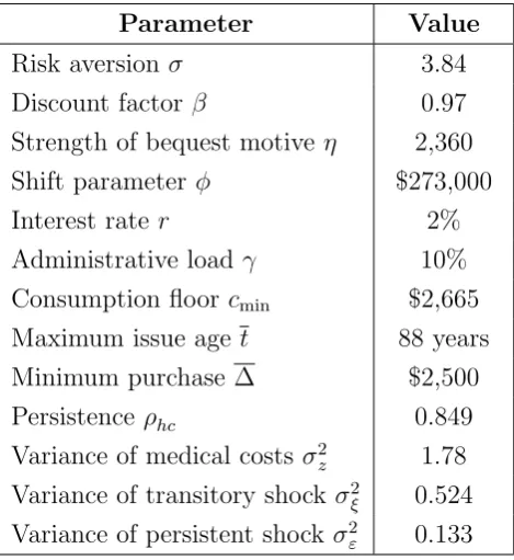
The annual interest rate r is set to 2%. The administrative load γ is assumed to be equal to 10%. This number is based on the study of Mitchell et al. (1999) which showed that on average, U.S. insurance companies add 10% to the annuity price because of administrative costs. The maximum issue age is set to be equal to 88 years. In general, the maximum issue age varies by state and ranges from 80 years old to the mid-90s (Levy et al, 2005).

The minimum purchase requirement is set to $2,500. This means that in order to buy an annuity, an individual should be willing to initiate a contract that will bring him at least $2,500 per year or $208 per month. Given prices produced by the model, this is equivalent to a minimum initial premium (q∆) of approximately $28,000 for a 70 year old and $12,000 for an 88 year old. This is in line with the restrictions on minimum premiums set by big annuity distributors such as Vanguard and Berkshire-Hathaway.

The parameters governing the evolution of health, survival, and medical expenses come from papers by DFJ and French and Jones (2004). The persistence parameter (ρhc) is set to 0.849. The innovation variance of the persistent component σ

2

ε is equal

to 0.133 and the innovation variance of the transitory component σ2

ξ is 0.524. The sum

of persistent and transitory components is normalized to one.8 _{The variance of the log}

medical expenses σ2

z is equal to 1.78.

8

DFJ’s estimates of the stochastic component of medical expenses are based on the results of French and Jones (2004). The difference between these two studies is that DFJ uses one year medical expenses while French and Jones (2010) use two-year averages. Since in my model one period is two years, I use French and Jones’s (2004) estimates and adjust the mean. The corresponding parameters for the one year process are: ρhc= 0.922,σ

2

ε= 0.050, andσ

2

For the discount factor β, preference parameters σ, η, and ϕ, and the minimum con-sumption floor cmin I use structural estimates from the DFJ study. In particular, β is

set to 0.97, σ to 3.84, and cmin to $2,665. The strength of the bequest motive η is set

to 2,360 and the shift parameter ϕ to $273,000.9

Table 1 summarizes all the parameter values.10

Parameter Value Risk aversionσ 3.84 Discount factorβ 0.97 Strength of bequest motive η 2,360 Shift parameter ϕ $273,000 Interest rater 2% Administrative loadγ 10% Consumption floorcmin $2,665

Maximum issue aget 88 years Minimum purchase ∆ $2,500 Persistenceρhc 0.849

Variance of medical costsσ2

z 1.78

Variance of transitory shock σ2

ξ 0.524

Variance of persistent shockσ2

ε 0.133

Table 1: Parameters of the model

4.2

Initial distribution

To calibrate the initial distribution of retirees over the state variablesk0, n0, m0 I use

the Health and Retirement Study (HRS) dataset. I use the RAND version of all the variables except for the annuity ownership rates. Individuals in the model start their retired life at age 70, so I used the cohort aged 65-75 in 1998 (wave 4) to calibrate the initial distribution.11

The sample used for simulations includes only single retirees.

9

The results for several alternative values of the coefficients of risk aversion, discount factor and bequest parameters are reported in Appendices A and B.

10

All parameters correspond to annual values except for parameters describing the evolution of stochas-tic medical expenses.

11

All Income quintiles

1st 2nd 3rd 4th 5th Mean

Age 70.4 68.8 70.7 70.6 71.0 70.7 Total wealth 161,311 70,942 78,213 173,047 197,731 287,082 Non-housing wealth 107,047 47,147 41,916 116,132 134,201 196,168 Income 12,964 4,403 7,766 10,667 14,820 23,206 Median

Age 71 68 71 71 72 71

Total wealth 64,000 3,000 22,500 71,000 112,000 176,950 Non-housing wealth 13,000 43 2,300 15,650 44,000 87,200 Income 10,663 4,773 7,802 10,671 14,720 23,725 Percent

Healthy 59.2 39.7 54.2 61.5 66.3 74.3 Own life annuity 5.0 0.4 1.0 5.3 6.4 12.2

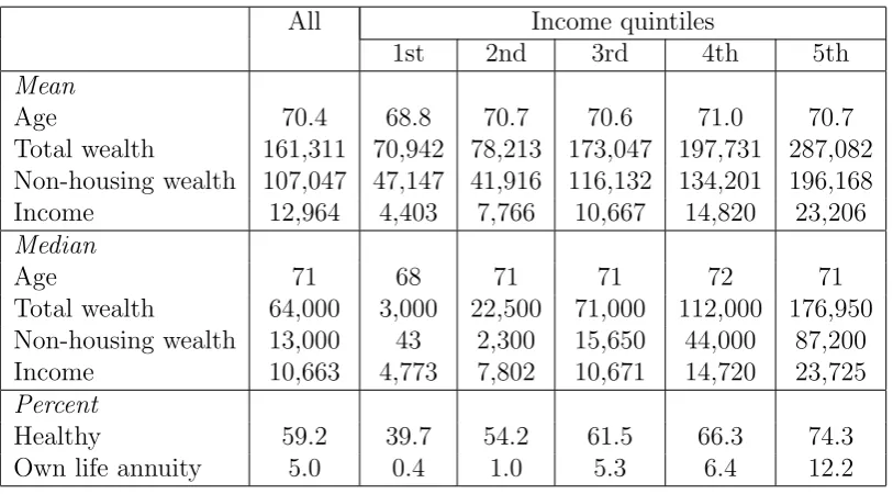
Table 2: Sample characteristics

Singles are defined as people who are divorced, never married or widowed and who reported having no partner. A person is defined as retired if his annual earnings were below $3,000. The resulting sample size is 1,483. I convert all dollar variables to constant 1998 dollars using the Consumer Price Index (CPI).

Initial wealth (k0) includes the value of housing and real estate, vehicles, value of

busi-ness, IRAs, Keoghs, stocks, bonds, checking, saving and money market accounts, minus mortgages and other debts. Preexisting annuity holdings (n0) correspond to annuity-like

income that an individual is entitled to receive during his retirement years and it also proxies permanent income (I). I follow DFJ in defining permanent income (or annuity-like income) as the sum of Social Security benefits, DB pensions, veteran benefits, food stamps, and annuities that individuals receive each year and then take the average over all years that individuals are observed in the data. Table 2 displays means and medians for the total and non-housing wealth and income in the sample used for simulations. The displayed statistics illustrate a substantial heterogeneity across income quintiles. People in the top quintile receive income that is on average almost five times higher than peo-ple in the bottom quintile. The disparity in wealth holdings is even more pronounced. Median total wealth of retirees in the bottom quintile is only $3,000, while for the top quintile it is close to $180,000.

Initial health (m0) is defined based on self-reported health. Individuals who report

fraction of healthy people in the bottom quintile (38%).

When constructing annuity ownership rates for my sample, I define a person as having life annuity if the following two conditions hold. First, he answers ’yes’ to the question of whether he receives income from an annuity other than pensions or Social Security. Second, he reports that at least one of his two largest private annuities continues for life. The resulting annuity ownership rates are shown in the last row of Table 2. Overall, only 5% of people own life annuities.12 _{There is a substantial heterogeneity in annuity market}

participation rates by income quintiles. While almost no retirees in the bottom quintile own annuities, in the top quintile the annuity ownership rate exceeds 12%.

5

Results

This section describes the model predictions about the annuity market participation rates and compares them to the data. To evaluate the combined effect of all factors behind non-annuitization I consider two versions of the model: the model that has no impediments to annutization (hereafter called the simple model), and the model with all seven impediments to annuitization (hereafter called the full model). The full model is as described in Section 3 (with asymmetric information equilibrium) while the simple model represents its stripped-down version where all features that can negatively affect the annuity demand are assumed away.

To evaluate the relative quantitative importance of different factors behind non-annuitization, I consider two sets of experiments. I start with the full model and remove impediments for annuitization one at a time, keeping all other model features constant. I then compare the annuity market participation rates between the full model and the model where one impediment to annuitization is missing. In the next set of experiments, I start with the simple model and I add different impediments to annuitization one at a time. Then I compare the annuity market participation rates between the simple model and the model where only one impediment to annuitization is present.

The experiments that switch on/off different factors affecting the annuity demand are designed in the following way.

Adverse selection. The model without adverse selection assumes symmetric informa-tion equilibrium in the annuity market , i.e. retirees face individually priced annuities. The model with adverse selection assumes asymmetric information equilibrium, i.e. there is only one pooling price for each age.13

12

The percentage of people who own both life and period-certain annuities constitutes 7.3%.

13

Consumption floor. The consumption floor cmin estimated by DFJ ($2,665) is on

the low side of what is commonly used in the literature (see Kitao and Jeske, 2009 and Kopecky and Koreshkova, 2011). In the model with high consumption floor this number is raised to $6,000.

Illiquid housing. In the model with illiquid housing initial wealth k0 is redefined as

total wealth minus housing wealth.14

Preannuitized wealth. In the model with preannuitized wealth retirees receive annuity-like incomen0 from Social Security and DB plans as observed in the data. In the model

without preannuitized wealth it is assumed that all annuity-like income is converted to liquid wealth. This conversion is done by assuming that individuals sell all annuity-like income they are entitled to receive at market prices for the case of symmetric information equilibrium.15

Minimum purchase requirements, medical expenses, and bequest motives. In the model without minimum purchase requirement ∆ is set to zero, i.e. people can buy any amount of annuities. In the model without medical expenseszt= 0 for allt. In the model without

bequest motives the strength of bequest η is set to zero.

5.1

Combined effect of all the impediments to annuitization

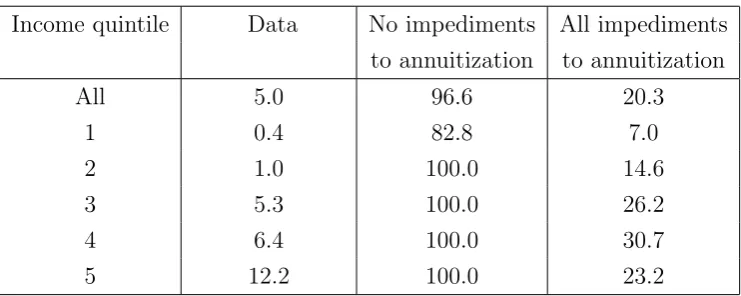
Table 3 compares annuity market participation rates for people at age 70 for the data, the simple model and the full model.16

The simple model predicts that almost 97% of people buy annuities. Those few people who do not participate in the annuity market come from the bottom income quintile: in this quintile 82.8% of people buy annuities, while in all other quintiles the participation rate is 100%. The non-participating indi-viduals are those who start retirement with almost zero wealth and who rely mostly on government means-tested transfers.

The full model goes a long way towards decreasing the annuity demand: once all potential explanations for the annuity puzzle are included, the participation rate drops from 97% to around 20%.17 _{However, it still remains higher than in the data (5%).}

medical expenses I only focus on equilibriums where people buy annuities only once in the first period. This does not affect the main results because the group that chooses to buy additional annuities later is very small.

14

Ideally, one would want to allow people to adjust their housing wealth inside the model. However, this involves adding another state variable which makes the model computationally intractable. To get some idea of the importance of housing wealth, I compare two extreme assumptions: i)housing has the same liquidity as other types of wealth, ii) housing is absolutely illiquid.

15

If I assume individuals sell preexisting annuities at prices observed under equilibrium with asym-metric information the resulting amount of liquid wealth will differ from one experiment to another due to the changing prices.

16

I show the participation rates only at age 70 because, as shown later, people start buying annuities in the first period of retirement and in most cases they do it once.

17

Income quintile Data No impediments All impediments to annuitization to annuitization

All 5.0 96.6 20.3

1 0.4 82.8 7.0

2 1.0 100.0 14.6

3 5.3 100.0 26.2

4 6.4 100.0 30.7

5 12.2 100.0 23.2

Table 3: Participation in the annuity market: data, model with no impediments to an-nuitization, and model with all impediments to annuitization

Section 5.4 discusses what changes in the benchmark calibration can move the model closer to the data.

5.2

Relative importance of different impediments to

annuitiza-tion

5.2.1 Analyzing the full model

The top panel of Table 4 shows how much annuity market participation rates change when only one impediment to annutization is removed from the full model. The most quantitatively important factor is preannuitized wealth. Elimination of this factor in-creases the annuity ownership rate more than twofold. If there is no preannuitized wealth around 42% of retirees will buy annuities even if all other impediments to an-nuitization are present. The next three most important factors are illiquid housing, minimum purchase requirement and bequest motives: without each of these factors the annuity ownership rates will be more than 35%. It is important to note that illiquidity of housing, preannuitized wealth and minimum purchase requirement act through a similar mechanism: they decrease the possibilities for annuitization. Annuities pay out for a long period of time and thus involve big upfront investments. Minimum purchase requirement increases these upfront costs, and illiquidity of housing and preannuitized wealth decrease the amount of wealth available for annuitization. This suggests that disposable wealth is an important factor affecting the demand for annuities, especially if there is a restriction on the minimum amount that can be invested.18

There is some heterogeneity in terms of how different impediments to annuitization affect people in different income quintiles. For the two bottom quintiles, illiquidity of

18

Income Full No adv. No med. Lowcmin No Liquid No min. No preann

quintile model selection expense bequest housing purchase wealth All 20.3 19.9 23.6 27.2 36.3 39.0 35.8 42.0

1 7.0 10.5 10.1 8.8 8.1 18.7 12.1 3.9

2 14.6 20.6 20.9 15.8 17.4 32.7 29.3 6.9 3 26.2 33.7 32.9 29.9 34.8 50.3 48.5 29.0 4 30.7 30.1 33.3 43.6 53.5 55.0 51.5 75.7 5 23.2 5.0 20.9 38.1 67.7 38.5 37.8 94.7

Income Simple + adv. + med. High cmin + Illiquid + min. + preann

quintile model selection expense bequest housing purchase wealth All 96.9 92.2 92.8 84.1 96.6 95.7 95.1 83.5

1 82.8 60.9 65.5 32.9 82.8 78.5 75.8 59.6 2 100.0 100.0 98.7 88.2 100.0 100.0 100.0 77.4 3 100.0 100.0 100.0 99.7 100.0 100.0 100.0 89.8 4 100.0 100.0 100.0 100.0 100.0 100.0 100.0 95.9 5 100.0 100.0 100.0 100.0 100.0 100.0 100.0 94.6

housing wealth has the largest quantitative impact on the fraction of annuity market participants. The removal of preannuitized wealth, however, decreases their demand for annuities. When Social Security and DB pension income is converted to liquid wealth, the annuity ownership rate for the bottom income quintile goes down from 7.2% to 3.9%. This happens because of the interaction of preannuitized wealth and a high consumption floor which will be discussed later when analyzing the simple model. For the top income quintile, the two most important factors affecting the annuity demand are preannuitized wealth and bequest motives. This happens because people in this group hold a large amount of preannuitized wealth and its transformation into liquid wealth has a large impact on resources available for annuitization. As for bequests, these are luxury goods and this strongly affects people in the top income quintile because they have higher wealth (see Table 2). Note that no other income quintile is affected by bequest motives to such an extent as the fifth quintile.

Another important observation from the top panel of Table 4 is that the removal of adverse selection from the full model has almost no impact on the overall annuity ownership rate. However, this hides a substantial heterogeneity in how this factor affects people in different income quintiles. In the absence of adverse selection there is a drop in the annuity market participation rate from the top two income quintiles and an increase in the participation from the bottom three quintiles.

The heterogeneous effect of adverse selection arises because the survival probability is positively correlated with income. In the asymmetric information equilibrium when annuities are priced only based on age, people in high income quintiles (and low survival probabilities) enjoy annuity prices that are lower than they would face if their survival probability was observed. In other words, higher income quintiles get an implicit subsidy from low income quintiles. Table 5 provides a quantitative assessment of this subsidy. For people in the lowest income quintile and in bad health, the pooling equilibrium price is around 57% higher than the price they face if insurance firms observe their mortality. At the other extreme, people in the highest income quintile and in good health pay almost 12% less for annuities than in the symmetric information equilibrium.

Note that the removal of medical expenses has a small effect on the overall annuity ownership rates. Without medical expenses the demand for annuities from the bottom and middle income quintiles goes up, while it decreases for the top quintile. The effect of medical expenses will be discussed in more detail later when I analyze the simple model.

5.2.2 Analyzing the simple model

Income quintile Bad health Good health

1 56.5 21.1

2 40.7 11.2

3 26.5 2.5

4 13.9 -5.1

5 3.2 -11.7

Table 5: Percentage change in price in the pooling equilibrium comparing to the sym-metric information equilibrium

impediment to annuitization has little power in decreasing annuity ownership rates: when the life-cycle model features only one factor that can potentially decrease the annuity demand the participation rate is always above 80%. This suggests that to explain low demand for annuities it is important to take into account the interaction between different factors behind non-annuitization.

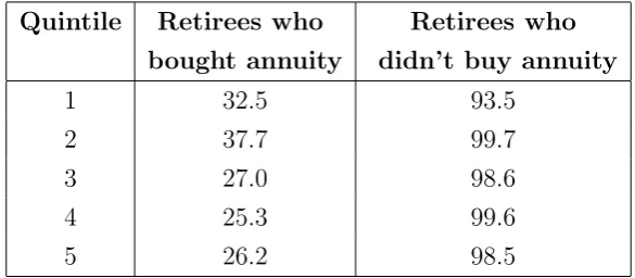
Two factors have the largest quantitative impact in the simple model: preannuitized wealth and the consumption minimum floor. Both factors decrease the demand for annuities from 97% to around 84%. However, the mechanism behind the effect of these two factors is different. Preannuitized wealth substantially decreases annuity market participation rates because many people have almost no financial resources except for Social Security and DB income. Table 6 illustrates this further by showing the share of annuity income in total amount of available resources n0

k0+n0

separately for people who bought annuities and those who did not in the simple model with preannuitized wealth. Those retirees who decide not to invest in annuities have few resources except for annuity income: the percentage of annuity income in total available funds is more than 90%. For people who chose to invest in annuities this percentage is much lower: it does not exceed 40%.

Quintile Retirees who Retirees who bought annuity didn’t buy annuity

1 32.5 93.5

2 37.7 99.7

3 27.0 98.6

4 25.3 99.6

5 26.2 98.5

Table 6: Average shares of annuity-like income in available resources

people who outlive their assets. In the presence of preannuitized wealth most people have pension income that exceeds the consumption floor. Once preannuitized wealth is converted to liquid wealth, people may use this opportunity to consume out of this liquid wealth and then rely on the consumption floor as opposed to buying private annuities. This strategy becomes more attractive as the consumption floor increases. In other words, when the consumption floor is high and there is no preannuitized wealth, low-income people have less incentives to buy annuities. This explains why the removal of preannuitized wealth from the full model decreases the demand for annuities from the lowest income quintiles as shown in the top panel of Table 4. This result also emphasizes the importance of taking into account the interaction between government means-tested transfers and preannuitized wealth when considering the consequences of the transition from Defined Benefits to Defined Contribution pension plans or possible privatization of Social Security.

Another important observation from the second panel of Table 4 is that except for preannuitized wealth, no other factor can affect all income quintiles. In the top two income quintiles everyone buys annuities regardless of what impediments to annuitization are present.

5.2.3 Sequential analysis

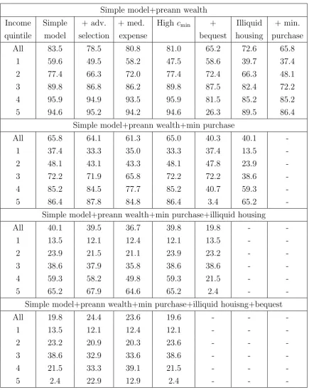
In the next set of experiments I cumulatively add to the simple model the four imped-iments to annuitization that turned out to be the most quantitatively important in the full model. The first panel of Table 7 considers the quantitative implications of adding one impediment to annuitization to the simple model that already features preannuitized wealth.

In this setup the impact of different factors becomes more pronounced. The two most important factors are now the minimum purchase requirement and bequest motives: each of these factors decreases the participation rate from around 84% to less than 66%. An-other important observation is that bequest motive introduces strong non-monotonicity in the relationship between the annuity market participation rate and income quintile. For example, in the presence of bequest motives only around 26% of people in the top income quintile buy annuities while among the third quintile the participation rate is around 82%. This goes in sharp contrast with the data, where the relationship between annuity ownership rates and income is strongly monotone (see the first column of Table 3). Notice also that in the model where retirees have preannuitized wealth the consump-tion floor has much less impact on the annuity market participaconsump-tion rate. This happens because most retirees have pension income which is above the consumption floor and thus this safety net does not impact their decisions to annuitize.

differ-Simple model+preann wealth

Income Simple + adv. + med. Highcmin + Illiquid + min.

quintile model selection expense bequest housing purchase All 83.5 78.5 80.8 81.0 65.2 72.6 65.8

1 59.6 49.5 58.2 47.5 58.6 39.7 37.4 2 77.4 66.3 72.0 77.4 72.4 66.3 48.1 3 89.8 86.8 86.2 89.8 87.5 82.4 72.2 4 95.9 94.9 93.5 95.9 81.5 85.2 85.2 5 94.6 95.2 94.2 94.6 26.3 89.5 86.4

Simple model+preann wealth+min purchase

All 65.8 64.1 61.3 65.0 40.3 40.1 -1 37.4 33.3 35.0 33.3 37.4 13.5 -2 48.1 43.1 43.3 48.1 47.8 23.9 -3 72.2 71.9 65.8 72.2 72.2 38.6 -4 85.2 84.5 77.7 85.2 40.7 59.3

-5 86.4 87.8 84.8 86.4 3.4 65.2

-Simple model+preann wealth+min purchase+illiquid housing

All 40.1 39.5 36.7 39.8 19.8 -

-1 13.5 12.1 12.4 12.1 13.5 -

-2 23.9 21.5 21.1 23.9 23.2 -

-3 38.6 37.9 35.8 38.6 38.6 -

-4 59.3 58.2 49.8 59.3 21.5 -

-5 65.2 67.9 64.6 65.2 2.4 -

-Simple model+preann wealth+min purchase+illiquid houisng+bequest

All 19.8 24.4 23.6 19.6 - -

-1 13.5 12.1 12.4 12.1 - -

-2 23.2 20.9 20.3 23.6 - -

-3 38.6 32.9 33.6 38.6 - -

-4 21.5 33.3 39.1 21.5 - -

-5 2.4 22.9 12.9 2.4 - -

ent impediments to annuitization in the simple model that already features preannuitized wealth and minimum purchase requirement. In this setup the strongest impact is pro-duced by illiquidity of housing wealth and bequest motives. In total, the combination of minimum purchase requirement, preannuitized wealth and one of these two factors can decrease the annuity ownership rates to 40%. This version of the model also highlights the interaction between the illiquidity of housing wealth and minimum annuity purchase requirement. When people face no restrictions on how much they can invest in annuities, the illiquidity of housing wealth has a moderate impact on the annuity demand (see the first panel of Table 7). However, once minimum purchase restriction is introduced, the illiquidity of housing wealth reinforces this constraint and substantially decreases the demand for annuities.

The third panel of Table 7 repeats the analysis for the model that already features illiquid housing, preannuitized wealth and minimum annuity purchase requirement. Con-sistent with the previous results, in this environment bequest motives stand out as the most important impediment to annuitization. In total the combination of bequest mo-tives, illiquid housing, preannuitized wealth and minimum annuity purchase requirement can reduce the demand for annuities to around 20%, which is the same as in the full model. However, as in the previous set of experiments, bequest motives result in non-monotone relationship between annuity ownership and income.

The last panel of Table 7 shows how adding adverse selection, medical expenses and increasing the consumption floor changes the demand for annuities in the model that already features bequest motives, minimum purchase requirement, illiquidity of housing and preannuitized wealth. In general, adding additional factors to the model that already features the four most powerful impediments to annuitization cannot decrease the annuity demand any further.

5.3

Life-cycle pattern of annuity purchase

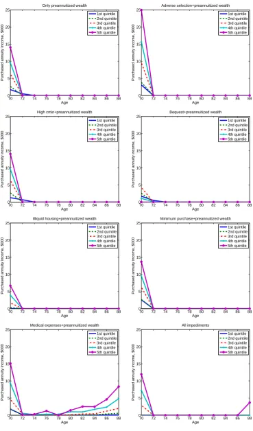
Figure (1) illustrates how age profiles of annuity purchases are affected by different impediments to annuitization. To highlight the importance of different factors the exper-iments are performed for the simple life-cycle model with preannuitized wealth.19 _The

patterns of annuity purchase are simulated for individuals who initially are in good health and who were given the initial wealth and annuity income that correspond to the median values of the initial distribution for each permanent income quintile.20

In most experiments people buy annuities only once in the first period. It can be shown (see Appendix G) that, under certain conditions, the one-time purchase of annu-ities in the first period can be a general result. The conditions under which this result holds include the following:

1) There is no uncertainty except the time of death 2) Medical expenditures are zero

3) β(1 +r)<1 4) n0 > cmin.

The last condition ensures that an individual is already guaranteed income that ex-ceeds the minimum consumption floor.21

The intuition behind this theoretical result is as follows. There are two ways to finance an annuity purchase: using financial wealth or existing annuity income. The second way would imply an increasing consumption profile, which is not optimal givenβ(1 +r)<1. Thus, if an individual buys an annuity, he will use his financial wealth; if an individual waits to buy annuities, he has to save in bonds. But this strategy is dominated by buying annuities from the start, because over the long-run an annuity brings a higher return.

The most noticeable changes in the life-cycle pattern of annuity purchase are intro-duced by medical expenses. People still buy annuities at the beginning of retirement but they also increase annuity holdings towards the end of life. This happens since retirees now have to finance not only their consumption but also medical expenditures that are increasing steeply over time. In this case, retirees use their annuity income to buy more annuities.

The bottom right graph in Figure (1) shows the life-cycle annuity purchase profile

19

The graphs look very similar for the case when there is no preannuitized wealth but the amount of annuity purchased is larger and the effect of each factor is less pronounced. On average, in the absence of preannuitized wealth people buy twice as much annuity income.

20

The graphs for individuals who start retirement in bad health are omitted because the patterns look the same except for the difference in the magnitude of purchase.

21

70 72 74 76 78 80 82 84 86 88 0 5 10 15 20 25 Age

Purchased annuity income, $000

Only preannuitized wealth

1st quintile 2nd quintile 3rd quintile 4th quintile 5th quintile

70 72 74 76 78 80 82 84 86 88

0 5 10 15 20 25 Age

Purchased annuity income, $000

Adverse selection+preannuitized wealth

1st quintile 2nd quintile 3rd quintile 4th quintile 5th quintile

70 72 74 76 78 80 82 84 86 88

0 5 10 15 20 25 Age

Purchased annuity income, $000

High cmin+preannuitized wealth

1st quintile 2nd quintile 3rd quintile 4th quintile 5th quintile

70 72 74 76 78 80 82 84 86 88

0 5 10 15 20 25 Age

Purchased annuity income, $000

Bequest+preannuitized wealth 1st quintile 2nd quintile 3rd quintile 4th quintile 5th quintile

70 72 74 76 78 80 82 84 86 88

0 5 10 15 20 25 Age

Purchased annuity income, $000

Illiquid housing+preannuitized wealth

1st quintile 2nd quintile 3rd quintile 4th quintile 5th quintile

70 72 74 76 78 80 82 84 86 88

0 5 10 15 20 25 Age

Purchased annuity income, $000

Minimum purchase+preannuitized wealth

1st quintile 2nd quintile 3rd quintile 4th quintile 5th quintile

70 72 74 76 78 80 82 84 86 88

0 5 10 15 20 25 Age

Purchased annuity income, $000

Medical expenses+preannuitized wealth

1st quintile 2nd quintile 3rd quintile 4th quintile 5th quintile

70 72 74 76 78 80 82 84 86 88

0 5 10 15 20 25 Age

Purchased annuity income, $000

All impediments 1st quintile 2nd quintile 3rd quintile 4th quintile 5th quintile

for the full model, i.e. the model with all the impediments to annuitization. Adding all other impediments to annuitization eliminates the pattern of increasing annuity pur-chases produced by medical expenses. In other words, medical expenses make it optimal for people to build up their income by annuitizing out of existing annuities, but other impediments to annuitization almost eliminate the demand for annuities for ages above 70.

5.4

Can the annuity market participation rate be decreased

further?

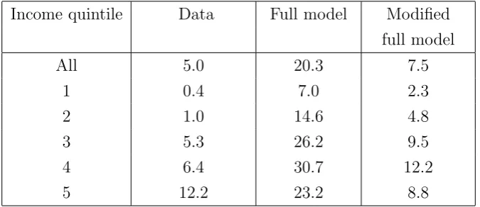
As Table 3 illustrates, even the full model with all the impediments to annuitization overpredicts annuity ownership rates comparing to the data. This section discusses in what directions the model can be modified in order to produce lower annuity demand.

The quantitative analysis above indicates that disposable wealth is one of the most important factors in determining the demand for annuities, especially when combined with minimum annuity purchase requirement. To understand whether these two factors are powerful enough to reduce the demand for annuities close to the level that we observe in the data, I introduce two modifications to the full model. First, I redefine the initial wealthk0by excluding from the total non-housing wealth the value of cars and businesses.

The motivation for this exercise is that given the special properties of these two types of assets it may be possible that retirees do not consider them as a potential target for annuitization. Second, I increase the minimum purchase requirement twice - from $2,500 to $5,000 annual annuity income. The results of this modified full model are reported in Table 8 alongside the data and the results from the original full model.

Income quintile Data Full model Modified full model

All 5.0 20.3 7.5

1 0.4 7.0 2.3

2 1.0 14.6 4.8

3 5.3 26.2 9.5

4 6.4 30.7 12.2

5 12.2 23.2 8.8

Table 8: Participation in the annuity market: data, full model and modified full model

that retirees own. If people consider all their assets equally suitable for annuitization, then it is hard to justify the observed low annuity demand. However, if people prefer not to annuitize their less liquid wealth then the standard life-cycle model augmented with high minimum purchase requirement and other impediments to annuitization can come close to accounting for low demand for annuities.

6

Conclusion

This study considers different explanations for the annuity puzzle in a quantitative heterogeneous agent model with equilibrium in the annuity market. It shows that in the absence of any impediments to annuitization all but the poorest retirees buy annuities. The life-cycle model that incorporates all impediments to annuitization decreases the de-mand for annuities almost five times. The most quantitatively important impediments to annuitization are preannuitized wealth, illiquid housing, minimum purchase requirement and bequest motives. Adverse selection noticeably decreases the demand for annuities amongst people in the bottom income quintiles but increases the demand from the top quintiles, thus producing a small overall effect. Medical expenses have a small effect on annuity ownership rates but they can substantially change the life cycle pattern of annuity purchases.

A

Alternative specifications of bequest motives

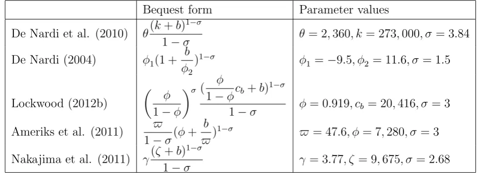
To understand how sensitive the demand for annuities to difference in bequest motives is, I use several alternative bequest specifications from the following studies: De Nardi (2004), Lockwood (2012b), Ameriks et al (2012) and Nakajima and Telyukova (2011). Bequest specifications for each of these studies are shown in Table 9 alongside with DFJ’s bequest specification that is used in the benchmark calibration (in Table 9 I keep the notation as in the original studies).

Bequest form Parameter values

De Nardi et al. (2010) θ(k+b)

1−σ

1−σ θ = 2,360, k = 273,000, σ= 3.84

De Nardi (2004) ϕ1(1 +

b ϕ2

)1−σ _ϕ

1 =−9.5, ϕ2 = 11.6, σ= 1.5

Lockwood (2012b)

(

ϕ

1−ϕ

)σ ( ϕ

1−ϕcb +b)

1−σ

1−σ ϕ= 0.919, cb = 20,416, σ= 3

Ameriks et al. (2011) ϖ

1−σ(ϕ+ b ϖ)

1−σ _{ϖ = 47.6, ϕ= 7,280, σ= 3}

Nakajima et al. (2011) γ(ζ+b)

1−σ

1−σ γ = 3.77, ζ = 9,675, σ = 2.68

Table 9: Bequest motives in various studies. Notation is the same as used by the authors,

b denotes the amount of wealth bequeathed

The parameterizations of bequest motives specified in Table 9 are not directly com-parable because each of these studies uses a different coefficient of risk-aversion and normalizes nominal variables to a different base year. To compare these bequest motives in the unified framework I use the following approach. First, I consider a simple one-period consumption-saving model augmented with a bequest motive. Assume an agent has wealth K. Tomorrow an agent dies with probability 1 and he can leave a bequest in the amountb. His consumption today will beK−b. The optimization problem looks as follows:

max

b {

(K−b)1−σ

1−σ +v(b)} (7)

The solution to this problem produces two outcomes: i) the threshold value of wealth above which a bequest motive becomes operational (K), i.e. people with wealth below the threshold will not leave a bequest22_{; ii) marginal propensity to bequeath (MPB), i.e.}

the fraction of each additional dollar of wealth that will be bequeathed once bequest is

operational. This can be defined as ∂b

∗

∂K where b

∗ _{is a solution to problem (7).}

22

K can be defined as follows: K= (v′₍₀₎₎−

1

Next, I compute the threshold and MPB implied by each bequest specification in Table 9. Both K and ∂b

∗

∂K are influenced not only by the parameters of bequest functions but

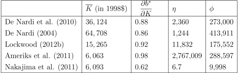
also by the risk aversion. In addition, the threshold values are nominal variables and thus depend on the base year used in each study. I convert them to one base year which is the same as used in my study. The resulting values for MPBs and for threshold values can be compared across studies and they are reported in the first two columns of Table 10. Note that the bequest motives under consideration cover a wide spectrum of possible bequest preferences. The least strong bequest motives (Nakajima and Telyukova, 2011) have MPB equal to 0.62, while the strongest bequest motives (Ameriks et al, 2011) have MPB equal to 0.98, which is equivalent to a linear bequest motive since almost the entire marginal wealth above the threshold is bequeathed. In terms of being luxury goods, the highest threshold among all specifications is $64,078 (De Nardi, 2004) while the lowest are $6,063 and $6,093 (Ameriks et al, 2011 and Nakajima and Telyukova, 2011). In other words, the form of De Nardi (2004) implies that bequests are luxury goods to a much larger extent than the forms of Ameriks et al (2011) and Nakajima and Telyukova (2011).

K (in 1998$) ∂b

∗

∂K η ϕ

De Nardi et al. (2010) 36,124 0.88 2,360 273,000 De Nardi (2004) 64,708 0.86 1,244 413,911 Lockwood (2012b) 15,265 0.92 11,832 175,552 Ameriks et al. (2011) 6,063 0.98 2,767,009 288,597 Nakajima et al. (2011) 6,093 0.62 6.7 9,998

Table 10: Bequest motives in various studies: unified framework

As a next step I need to find bequest parameters η and ϕ that can produce the same thresholds and MPBs as listed in Table 10 when plugged into the bequest function

υ(kt) =η

(ϕ+kt) 1−σ

1−σ together with the risk aversion used in my benchmark calibration.

The resulting values of η and ϕ are shown in the last two columns of Table 10. Next I solve four versions of the full model with these parameters of the bequest function. The results are shown in Table 11.

Income quintile DFJ De Nardi Lockwood Ameriks Nakajima (2010) (2004) (2012b) (2009) (2011)

All 20.3 34.8 0.0 0.0 25.8

1 7.0 7.9 0.0 0.0 8.1

2 14.6 17.4 0.0 0.0 11.3

3 26.2 34.2 0.0 0.0 27.4

4 30.7 53.4 0.0 0.0 35.6

5 23.2 61.3 0.0 0.0 46.6

Table 11: Annuity market participation rates for the full model with different parame-terizations of bequest motives.

bequest motives (see the top panel of Table 4). Even though the MPB in the bequest specification of De Nardi (2004) is almost the same as the MPB used in my benchmark calibration, the former bequest motives have a higher threshold and thus affect fewer peo-ple. Another important observation is that the bequest parametrization of Nakajima and Telyukova (2011) can reproduce the monotone relationship between annuity ownership and income.

Income quintile MPB=0.62 MPB=0.7 MPB=0.8 MPB=0.88 (original) (as in DFJ)

All 25.8 22.3 13.9 0.8

1 8.1 7.1 5.6 0.3

2 11.3 9.5 6.0 0.0

3 27.4 23.5 17.2 0.8

4 35.6 30.8 20.7 2.0

5 46.6 40.6 20.4 0.8

Table 12: Annuity market participation rates for the bequest parametrization of Naka-jima and Telyukova (2011) with higher MPB

B

Alternative specification of other preference

pa-rameters

This section checks the sensitivity of results to changes in two parameters: discount factor (β) and risk aversion (σ). The first two columns of Table 13 display participation rates in the annuity market for the full model when β is first raised to 0.98 and then decreased to 0.90. Note that in the first experiment β was increased to the point when

β(1 +r) = 1.

Income quintile Full model β = 0.98 β= 0.90 σ = 3 σ = 6 All 20.3 20.9 7.1 13.9 27.6

1 7.0 6.7 4.5 4.2 7.9

2 14.6 13.9 6.0 9.7 17.2

3 26.2 26.7 14.5 20.4 32.9 4 30.7 33.1 7.5 22.5 43.7 5 23.2 24.0 3.0 12.6 36.1

Table 13: The sensitivity of annuity ownership rates to changes in the discount factor and the risk aversion

A decrease in the discount factor decreases annuity market participation rates while an increase in the discount factor has almost no effect. Impatient individuals save less and so they are less interested in annuities: when the discount factor goes down to 0.90, the participation rate drops more than twofold.

experiments. When the risk aversion decreases, agents want to save less and thus they buy less annuities.23

An increase in the risk aversion has the opposite effect, thus higher risk aversion makes the annuity puzzle harder to explain.

C

Alternative specifications for the administrative

loads

When modeling the annuity market I made the assumption that the administrative load is proportional to the amount of insurance sold. This section shows how this as-sumption can affect the results. To do this I consider an alternative specification for the administrative costs by assuming they do not depend on the total value of insurance contract but represent fixed additive costs. In this case equation (4) can be rewritten as follows:

πt(Ωt) =qt(Ωt)− T−t

∑

i=1

b

St+i|t(Ωt)

(1 +r)i −eγ (8)

where _eγ is lump sum administrative costs.

To be consistent with the results of Mitchell et al (1999) I set _eγ so that the fraction of administrative costs in the total value of the contract is equal to 10% for people of age 70. The results of the full model with this alternative specification of administrative costs is reported in Table 14. Comparing to the full model with proportional administrative costs, annuity ownership rates are very similar.

Income quintile Full model Additive load

All 20.3 19.7

1 7.0 6.9

2 14.6 13.9

3 26.2 26.2

4 30.7 29.8

5 23.2 21.8

Table 14: The sensitivity of annuity ownership rates to the different specification of ad-ministrative loads

23

D

Equilibrium annuity prices

This section compares prices produced by the full model with the prices observed in the data. Figure 2 shows that prices in the model line up well with what we see in the data24_{, though for most ages the model underpredicts the real prices.}

70 72 74 76 78 80 82 84 86 88

4 5 6 7 8 9 10 11 12 13

Age

Price, $

Price for unit of insurance contract ($)

Model Data

Figure 2: Prices in the full model and in the data

There are at least three explanations for this downward bias of the prices in the model. First, the model considers only single individuals, while real prices are based on the aggregate statistics that include couples. Second, the HRS dataset underrepresents wealthy individuals. Given that wealth is negatively correlated with mortality and that rich individuals tend to buy more annuities, the lack of wealthy individuals in the model biases the prices downwards. Third, this paper makes an assumption that insurance firms are perfectly competitive and sets administrative load to 10%. It may be that the markup insurance firms set is more than 10% due to higher administrative expenses or violation of the perfect competition assumption.

E

Annuitization levels

This section discusses how different factors affect the optimal level of annuitization. Table 15 shows the median fractions of liquid wealth annuitized by retirees in the sim-ple model that features preannuitized wealth. When there is no other impediment to annuitization except Social Security and DB plans, median annuitization level is 60% for retirees in the bottom quintile and around 82% for the top income quintile. Most

24

impediments strongly affect people in the bottom quintile. Medical expenses decrease their median annuitization level to less than 10%, while in the presence of adverse selec-tion, high consumption floor, illiquidity of housing and minimum purchase requirement median annuitization level of this group becomes zero. For the top income quintile the strongest impact is produced by bequest motives, which result in zero annuitization level. Illiquidity of housing and minimum purchase requirement have very small negative im-pact on the optimal annuitization level for this group. Medical expenses and adverse selection actually increase the fraction of wealth annuitized in the top income quintile.

Income Simple + adv. + med. Highcmin + Illiquid + min.

quintile model selection expense bequest housing purchase

1 59.3 0.0 9.7 0.0 39.2 0.0 0.0

2 76.6 66.1 51.5 76.1 50.7 46.4 0.0 3 80.0 79.5 75.4 80.0 36.8 74.1 79.8 4 81.5 82.5 81.8 81.0 14.8 78.9 81.2 5 81.9 83.9 87.3 81.9 0.0 79.1 78.5

Table 15: Median fraction of liquid wealth annuitized in the simple model with preannu-itized wealth

F

Welfare

Another dimension to consider is how each impediment to annuitization changes people’s valuation of annuities. Table 16 illustrates the welfare gains of people from having access to the annuity market. Welfare gains are measured as the consumption equivalent variation (CEV). This represents the percentage of the annual consumption that a retiree who does not have access to the annuity market is willing to give up in order to get an option to buy annuities. The results are presented for the simple model with preannuitized wealth. Overall, if there are no impediments to annuitization except for Social Security and DB plans, gaining access to the annuity market is equivalent to increasing consumption by 2% each period. People in high income quintiles gain more than people in low quintiles since they have more wealth to invest in annuities and hence can change their consumption patterns in a more significant way when the annuity market is available.

Income Only prean + adv. + med. High cmin + Illiquid + min.

quintile wealth selection expense bequest housing purchase

All 2.0 1.1 1.6 2.5 1.6 0.7 1.7

1 1.7 0.8 1.1 1.8 1.6 0.5 1.4

2 2.8 1.7 1.7 2.8 1.8 1.2 2.4

3 4.8 3.9 3.8 4.8 1.6 2.1 4.6

4 5.8 6.0 6.7 5.7 0.4 2.5 5.6

5 4.5 6.1 8.6 4.6 0.0 2.3 4.4

Table 16: Consumption equivalent variation for the simple model with different impedi-ments to annuitization

decreases the CEV from 2.0% to 1.1%. The effect of adverse selection on the annuity valuation is positive for people in high income quintiles and negative for people in low income quintiles, and the latter effect dominates. Similar effects are produced by medical expenses: the CEV for high-income groups goes up while for low-income groups it goes down. People in high quintiles value annuities more since they can use them to insure against uncertain medical expenses. For low income quintiles medical expenses substan-tially increase the risk of falling under the consumption minimum floor, and in this state annuities do not have any value.

Another factor that has a heterogeneous effect on different income quintiles is bequest motives, which have almost no effect on the bottom quintiles but decrease the CEV of the highest income quintile to almost zero.

Surprisingly, higher consumption minimum floor increases the value of the annuity market from 2.0% to 2.5% and this happens because of the change in the CEV of low-income group. This is mostly driven by a change in the welfare of people whose preexisting annuity income is below the high consumption floor, and without an annuity market they quickly decumulate their assets and rely on government transfers. After gaining access to the annuity market they can increase their annuity income above the level ofcmin and

this gives them higher lifetime consumption.

G

Theory

G.1

Auxiliary propositions

Auxiliary proposition 1 Assume there is no uncertainty except the time of death. Then the following is true:

1 +qAF t+1

qAF t

= 1 +r

st

where qAF

t is an actuarially fair annuity price defined as follows:

qAF t =

T−t

∑

i=1

St+i|t

(1 +r)i

Proof Using the definition of actuarially fair annuity prices and the fact thatSt+i|t=

stSt+i|t+1 we can write:

qtAF =

st

(1 +r) (

1 +

T−t

∑

i=2

St+i|t+1

(1 +r)i−1 )

= st (1 +r)

(

1 +qAFt+1

)

This proves Auxiliary proposition 1.

Auxiliary proposition 2 Assume there is no uncertainty except the time of death. Then the following is true:

1 +qt+1

qt

< 1 +r st

where qt is the annuity price that includes administrative load, i.e. qt =γqtAF.

Proof We can write the following relationship:

1 +qt+1

qt

= 1 +γq

AF t+1

γqAF t

= 1/γ+q

AF t+1

qAF t

< 1 +q

AF t+1

qAF t

The last inequality follows from the fact that γ ≥ 1. By Auxiliary proposition 1 1 +qAF

t+1

qAF t

= 1 +r

st

. Thus 1 +qt+1

qt

< 1 +r st

, which proves Auxiliary proposition 2.

G.2

Assumptions

The proofs below rely on the following assumptions: 1. There is no uncertainty except the time of death. 2. Medical expenses are zero (zt=0).

4. Annuity prices satisfy the following condition: 1 +qt+1

qt

>1 +r.25

5. The initial annuity income is above the consumption floor (n0 > cmin. )

6. There are no bequest motives.

G.3

Proof that people buy annuities only once in the first

pe-riod

Proposition 1 Assume conditions 1-5 hold. Then if an agent’s optimal investments in annuities at timet+ 1 is positive (∆t+2 >0) then he does not invest in bonds at time

t (kt+1 = 0).

Proof Suppose not. Consider Euler equations for an agent’s investments in annu-ities and bonds at time t. Given assumptions 5 and 6 we can write these equations as follows:

u′(ct)qt−µnt =βstu′(ct+1)(1 +qt+1)−µnt+1 (9)

u′(ct)−µkt =βst(1 +r)u′(ct+1) (10)

Hereµn

t and µkt are Lagrange multipliers on constraints ∆t+1 ≥0 andkt+1 ≥0 and they

satisfy the following conditions:

µnt ≥0, µ n

t∆t+1 = 0

µk

t ≥0, µktkt+1 = 0

Since ∆t+2 >0, we have µnt+1 = 0. By supposition, µkt = 0. Thus equations (9) and

(10) can be rewritten in the following way:

µn t

qt

=u′(ct)−βstu′(ct+1)

1 +qt+1

qt

u′(ct) = βst(1 +r)u′(ct+1)

Combining these equations we get:

µn t

qt

=βstu′(ct+1)

(

(1 +r)− 1 +qt+1

qt

)

Given assumption 4 this implies µn

t <0 which contradicts the definition of Lagrange

multiplier. This contradiction proves Proposition 1.

25