Munich Personal RePEc Archive
Estimating risk attitudes in conventional
and artefactual lab experiments
Drichoutis, Andreas and Koundouri, Phoebe
Dept. of Economics, University of Ioannina
January 2011
Online at
https://mpra.ub.uni-muenchen.de/28438/
1
Estimating risk attitudes in conventional and artefactual lab experiments
Andreas C. Drichoutis1 and Phoebe Koundouri2
1
Dept. of Economics, University of Ioannina, University campus, Ioannina, Greece, email: [email protected], tel: +30-26510-05954, corresponding author
2
Dept. of International and European Economic Studies, Athens University of Economics and Business, 76 Patision st., 10434, Greece, email: [email protected]
Abstract
We elicit and compare risk preferences from student subjects and subjects drawn from the general population, using the multiple price list method devised by Holt and and Laury (2002). We find evidence suggesting that students have lower relative risk aversion than others.
Keywords: Risk aversion, CRRA, expo-power, multiple price list
JEL codes: C91, D01, D81
1. Introduction
Economic lab experiments have been mainly performed in academic environments and students have therefore posed as the natural standard subject pool. Whether student samples provide a reliable sample for extrapolating results to the general population is an issue that is heavily criticized. Concerns on the use of students as research surrogates for consumers or adults in general, is rather old (Enis et al., 1972; McNemar, 1946). Reasons are attributed to the fact that students exhibit psychological, social and demographical differences from other segments of the population but also to the fact that students are not yet complete personalities.
2
student subject pool) and an artefactual lab experiment (i.e, using a general population subject pool).
2. Experimental data
We compiled data from two previous experiments that involved risk preference elicitations tasks. These two experiments were part of a larger project on choice under risk which also involved some standard experimental auction tasks. Experimental instructions for the experiments are available at https://sites.google.com/site/riskprefs/ . The first experiment used a student subject pool while the second experiment used a subject pool drawn from the general population. General population subjects were recruited by a professional company. The same proctor was used in both experiments.
In the student subject pool experiment, the purpose was to explore whether risk preferences can be manipulated by some treatment variables, so we only used data from the control treatment sessions. In the consumer subject pool experiment, risk preferences were not part of the experimental manipulation. In all, we used elicited risk preferences from 34 general population subjects and 23 student subjects. In the student subject pool experiment, in one session the auction task was placed after risk elicitation. For all other subjects, risk elicitation followed the auction. We use a dummy variable in our econometric estimation to control for this session-specific characteristic.
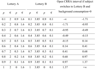
To elicit risk preferences we used the multiple price list (MPL) design devised by Holt and Laury (2002). In this design each subject is presented with a choice between two lotteries, A or B as illustrated in Table 1. In the first row the subject is asked to make a choice between lottery A, which offers a 10% chance of receiving €2 and a 90% chance of receiving €1.6, and lottery B, which offers a 10% chance of receiving €3.85 and a 90% chance of receiving €0.1. The expected value of lottery A is €1.64 while for lottery B it is €0.475, which results in a difference of €1.17 between the expected values of the lotteries. Proceeding down the table to the last row, the expected values of the lotteries increase but increases much faster for lottery B.
3
3. Estimation and Results
To estimate risk attitudes and assess the importance of the sample type as well as the demographics on risk preferences, we follow similar procedures to Holt and Laury (2002) and Harrison, et al. (2007).
Let the utility function be the constant relative risk aversion (CRRA) specification:
1 1 r M U M r (1)
for r≠1, where r is the CRRA coefficient. In (1), r=0 denotes risk neutral behavior, r>0 denotes risk aversion behavior and r<0 denotes risk loving behavior.
The binary choices of the subjects in the risk preference tasks can be explained by different CRRA coefficients (as reported in Table 1).
If we assume that Expected Utility Theory holds for the choices over risky alternatives, the likelihood function for the choices that subjects make can be written for each lottery i as:
1,2
i j j
j
EU p M U M
(2)where p M
j are the probabilities for each outcome Mj that are induced by the experimenter. To specify the likelihoods conditional on the model, the Luce stochastic specification is used. The expected utility (EU) for each lottery pair is calculated for candidate estimate of r,and the ratio:1 1 1 B A B
EU
EU
EU
EU
(3)is then calculated where EUA and EUB refer to options A and B respectively, and is a structural noise parameter. The index in (3) is linked to observed choices by specifying that the option B is chosen when 1
2
EU
.
The conditional log-likelihood can then be written as:
ln RA , ; , ln | 1 ln 1 | 1
i i
i
L r y X
EU y EU y (4)where yi 1
1 denotes the choice of the option B (A) lottery in the risk preference task i. Each parameter in equation (4) is allowed to be a linear function of demographic and treatment variables as exhibited in Table 2. A portion of subject’s fees was stochastic since this have been demonstrated to be very important for recruitment (Harrison et al., 2009). In addition, recruitment practices necessitated a higher show-up fee for consumer subjects. Thus, a total fee endowment variable is included in the econometric model. Equation (4) is maximized using standard numerical methods.4
general population subjects appear more risk averse than the student sample and the difference is highly significant.
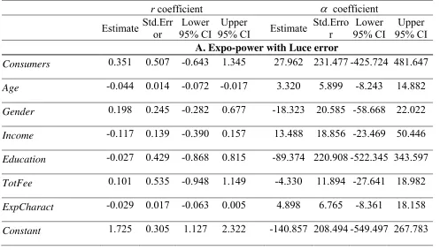
The CRRA characterization of risk preferences, while popular, restricts relative risk aversion to be constant over the prize domain. To allow for the possibility that the relative risk aversion is not constant we adopt a more flexible functional form; the hybrid expo-power
function of Saha (1993). The expo-power function can be defined as
1 exp
1r
u M aM a,
where M is income and
a
andr
are parameters to be estimated. Relative risk aversion (RRA) is then
11 r
ra r M . Results assuming the expo-power form are presented in Table 4 (panel A). It is obvious that by allowing a more flexible functional form the coefficient of the relevant sample type dummy is no longer statistically significant for neither
a
orr
. The magnitude of ther
coefficient is reduced as well.The Luce error popularized by Holt and Laury (2002), however, implicitly imposes a stochastic identifying restriction that the true stochastic model is CRRA-neutral (Wilcox, 2008). Different stochastic models should then be evaluated. Therefore, we also test the Fechner
specification (as in Harrison and Rutstrom, 2008), which posits EU EUB EUA
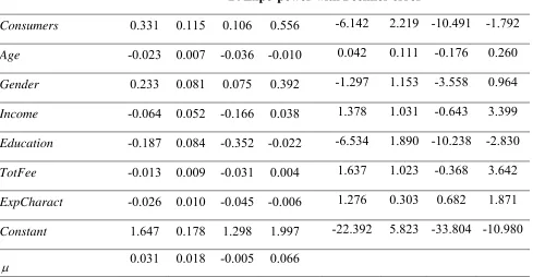
instead of
(3). Results for the CRRA and expo-power functions are exhibited in panels B in Table 3 and 4 respectively. The estimates for the Consumer dummy for
r
are statistically significant, positive and remarkably close to the expo-power with Luce error specification estimate. The estimate fora turns negative and is statistically significant.
So which specification should we trust? A non-nested hypothesis test like the Vuong (1989) test is appropriate in this context. The expo-power with Fechner error specification is favored in all cases [Vuong statistic: 2.07 (vs. expo-power Luce), 3.69 (vs. CRRA-Luce), 5.00 (vs. CRRA-Fechner)]. In the expo-power with Fechner error specification the negative coefficient of the relevant dummy for
a
(-6.142) implies lower RRA for general population subjects as compared to the student sample, ceteris paribus. In addition, the average prediction fora
is positive for both subsamples, indicating increasing RRA. Given a positivea
, the coefficient of the Consumers dummy forr
(0.331) implies a lower RRA for subjects of the general population as compared to students, ceteris paribus.Table 5 exhibits RRA predictions for the two subject pools for M=1 and M=5. The predictions indicate higher RRA for general population subjects and lower RRA for students. At a first glance this may seem like contrasting with the previous paragraph but should be of no surprise given the sign of the Age coefficients and the age difference between subject pools.
4. Conclusions
5
previous studies have either found no difference in risk aversion between students and the general adult population (Andersen et al., 2010a) or that students are more risk averse (Andersen et al., 2010b). This finding has significant implications for conventional laboratory experiments practice given the importance of risk preferences in everyday economic decision making. More studies that will examine differences in risk preferences between students and the general population are indeed warranted.
5. References
Andersen, S., G.W. Harrison, M.I. Lau, E.E. Rutström, 2010a. Discounting behavior: A reconsideration. working paper.
Andersen, S., G.W. Harrison, M.I. Lau, E.E. Rutström, 2010b. Preference heterogeneity in experiments: Comparing the field and laboratory. Journal of Economic Behavior and Organization 73, 209-224.
Barsky, R.B., F.T. Juster, M.S. Kimball, M.D. Shapiro, 1997. Preference parameters and behavioral heterogeneity: An experimental approach in the health and retirement study. Quarterly Journal of Economics 112, 537-579.
Enis, B.M., K.K. Cox, J.E. Stafford, 1972. Students as subjects in consumer behavior experiments. Journal of Marketing Research 9, 72-74.
Harrison, G.W., E. Johnson, M.M. McInnes, E.E. Rutström, 2005. Risk aversion and incentive effects: Comment. The American Economic Review 95, 897-901.
Harrison, G.W., M.I. Lau, E.E. Rutstrom, 2007. Estimating risk attitudes in Denmark: A field experiment. Scandinavian Journal of Economics 109, 341–368.
Harrison, G.W., M.I. Lau, E.E. Rutström, 2009. Risk attitudes, randomization to treatment, and self-selection into experiments. Journal of Economic Behavior & Organization 70, 498-507. Harrison, G.W., E.E. Rutstrom, 2008. Risk aversion in the laboratory, in: Cox, J.C., Harrison, G.W. (Eds.), Research in Experimental Economics Vol 12: Risk Aversion in Experiments. (Emerald Group Publishing Limited, Bingley, UK), pp. 41-196.
Holt, C.A., S.K. Laury, 2002. Risk aversion and incentive effects. The American Economic Review 92, 1644-1655.
Koundouri, P., M. Laukkanen, S. Myyrä, C. Nauges, 2009. The effects of EU agricultural policy changes on farmers' risk attitudes European Review of Agricultural Economics 36, 53-77.
Koundouri, P., C. Nauges, V. Tzouvelekas, 2006. Technology Adoption under Production Uncertainty: Theory and Application to Irrigation Technology. American Journal of Agricultural Economics 88, 657-670.
McNemar, Q., 1946. Opinion-attitude methodology. Psychological Bulletin 43, 289-374.
Saha, A., 1993. Expo-power utility: A flexible form for absolute and relative risk aversion. American Journal of Agricultural Economics 75, 905-913.
Vuong, Q.H., 1989. Likelihood ratio tests for model selection and non-nested hypotheses. Econometrica 57, 307-333.
6
Economics Vol 12: Risk Aversion in Experiments. (Emerald Group Publishing Limited, Bingley, UK), pp. 197-292.
7
Table 1. Sample payoff matrix for the risk preferences tasks
Lottery A Lottery B Open CRRA interval if subject switches to Lottery B and
background consumption=0
p € p € p € p €
0.1 2 0.9 1.6 0.1 3.85 0.9 0.1 -∞ -1.71
0.2 2 0.8 1.6 0.2 3.85 0.8 0.1 -1.71 -0.95
0.3 2 0.7 1.6 0.3 3.85 0.7 0.1 -0.95 -0.49
0.4 2 0.6 1.6 0.4 3.85 0.6 0.1 -0.49 -0.15
0.5 2 0.5 1.6 0.5 3.85 0.5 0.1 -0.15 0.14
0.6 2 0.4 1.6 0.6 3.85 0.4 0.1 0.14 0.41
0.7 2 0.3 1.6 0.7 3.85 0.3 0.1 0.41 0.68
0.8 2 0.2 1.6 0.8 3.85 0.2 0.1 0.68 0.97
0.9 2 0.1 1.6 0.9 3.85 0.1 0.1 0.97 1.37
1 2 0 1.6 1 3.85 0 0.1 1.37 +∞
Note: Last two columns showing implied CRRA intervals were not shown to subjects.
Table 2. Variable description
Variable Description
General population
subject pool Student subject pool
Mean Std.dev. Mean Std.dev.
Age Subject’s age 41.176 10.376 20.739 1.322
Gender Dummy, 1=males, 0=females 0.324 0.475 0.391 0.499
Income
Dummy, household’s economic position is above
average=1, else=0
0.471 0.507 0.435 0.507
Education Dummy, university graduate
or higher=1, else=0 0.676 0.475 0 0
TotFee Total fee endowment 23.794 6.594 16.717 1.146
ExpCharact
Dummy, risk preference task was conducted after an auction, else=0
[image:8.612.66.553.450.675.2]8
Table 3. Estimates of risk preferences (CRRA function)
r coefficient
Estimate Std.Err or
Lower 95% CI
Upper
95% CI Estimate
Std.Err or
Lower 95% CI
Upper 95% CI
A. CRRA with Luce error B. CRRA with Fechner error
Consumers 0.878 0.268 0.352 1.404 0.345 0.084 0.180 0.511
Age -0.038 0.015 -0.067 -0.008 -0.017 0.004 -0.025 -0.009
Gender -0.011 0.262 -0.525 0.503 -0.081 0.057 -0.193 0.032
Income 0.070 0.188 -0.299 0.439 0.062 0.043 -0.022 0.146
Education -0.311 0.217 -0.735 0.114 -0.099 0.063 -0.222 0.024
TotFee -0.138 0.262 -0.651 0.375 -0.149 0.052 -0.251 -0.047
ExpCharact -0.041 0.011 -0.063 -0.019 -0.009 0.005 -0.018 0.000
Constant 1.831 0.278 1.286 2.376 1.259 0.119 1.026 1.491
0.328 0.053 0.224 0.431 0.140 0.051 0.040 0.240
Table 4. Estimates of risk preferences (expo-power function)
r coefficient coefficient
Estimate Std.Err or
Lower 95% CI
Upper
95% CI Estimate
Std.Erro r
Lower 95% CI
Upper 95% CI
A. Expo-power with Luce error
Consumers 0.351 0.507 -0.643 1.345 27.962 231.477 -425.724 481.647
Age -0.044 0.014 -0.072 -0.017 3.320 5.899 -8.243 14.882
Gender 0.198 0.245 -0.282 0.677 -18.323 20.585 -58.668 22.022
Income -0.117 0.139 -0.390 0.157 13.488 18.856 -23.469 50.446
Education -0.027 0.429 -0.868 0.815 -89.374 220.908 -522.345 343.597
TotFee 0.101 0.535 -0.948 1.149 -4.330 11.894 -27.641 18.982
ExpCharact -0.029 0.017 -0.063 0.005 4.898 6.765 -8.361 18.158
[image:9.612.52.549.430.713.2]9
0.317 0.056 0.207 0.427
B. Expo-power with Fechner error
Consumers 0.331 0.115 0.106 0.556 -6.142 2.219 -10.491 -1.792
Age -0.023 0.007 -0.036 -0.010 0.042 0.111 -0.176 0.260
Gender 0.233 0.081 0.075 0.392 -1.297 1.153 -3.558 0.964
Income -0.064 0.052 -0.166 0.038 1.378 1.031 -0.643 3.399
Education -0.187 0.084 -0.352 -0.022 -6.534 1.890 -10.238 -2.830
TotFee -0.013 0.009 -0.031 0.004 1.637 1.023 -0.368 3.642
ExpCharact -0.026 0.010 -0.045 -0.006 1.276 0.303 0.682 1.871
Constant 1.647 0.178 1.298 1.997 -22.392 5.823 -33.804 -10.980
[image:10.612.55.544.111.365.2] 0.031 0.018 -0.005 0.066
Table 5. Relative risk aversion predictions based on expo-power function with Fechner error
Consumers Students
M=1 2.71 1.06