Munich Personal RePEc Archive
Estimation of a simple genetic algorithm
applied to a laboratory experiment
Alfarano, Simone and Eva, Camacho and Josep, Domènech
April 2010
Online at
https://mpra.ub.uni-muenchen.de/24138/
algorithm applied to a laboratory
experiment
Simone Alfarano1
, Eva Camacho Cuena2
, and Josep Dom`enech S`oria3
Abstract The aim of our contribution relies on studying the possibility of implementing a genetic algorithm in order to reproduce some characteristics of a simple laboratory experiment with human subjects. The novelty of our paper regards the estimation of the key-parameters of the algorithm, and the analysis of the characteristics of the estimator.
1 Introduction
Nowadays, a large part of economists expresses dissatisfaction (or sometimes rejection) to the wide-spread paradigm of full or strict rationality in theoriz-ing the behavior of economic agents. Laboratory experiments showed that, even in simple settings, human subjects are not consistent with the assump-tions implied by their supposed perfect rationality. An existing alternative paradigm in economic theory considers that economic agents have limited capabilities in processing the information and in taking their decisions. Con-trary to the fully rational paradigm, it does not exists a unified theory of bounded rationality. Therefore, many different models of human behavior which account for bounded rationality have been proposed in the literature (See for example [3]).
The adaptation of genetic algorithms (GA) from the realm of optimization literature to the description of human learning is an example of the creative ability of researchers to introduce bounded rational models.1
A number of papers are now available in the literature which apply different versions of GAs in order to reproduce the behavior of economic agents in different con-texts (See, for example, [9], [1], [2], [7]). GAs have also been applied in the
1
For more details on GA and their application to Economics see [6].
2 Simone Alfarano, Eva Camacho Cuena, and Josep Dom`enech S`oria
context of laboratory experiments in order to reproduce the human subjects’ behavior in different experimental settings (See [10], [4]).
However, up to now the different contributions are almost entirely based on a rough calibration of the underlying crucial parameters. To the best of our knowledge, our paper constitutes the first attempt to estimate the underlying parameters of a genetic algorithm. In this paper we provide a method to estimate the key parameters of the GA by means of an extensive simulation-based approach, using an extremely simple experimental setting of a common-pool resources problem.The experiment exhibits, in fact, a single dominant and symmetric Nash equilibrium as illustrated in the next section. The paper is organized as follows: in section 2 we illustrate briefly the the-oretical and empirical results of the experimental setting. In section 3 we detail the characteristics of the implementation of our GA agents. In section 4 we present the estimation procedure. Finally, in section 5 we conlcude.
2 Experiment: Setting and Results
In this section we will summarize the experimental setting and main results used as benchmark in order to build the GA and the corresponding parame-ters estimation.(See [5] for the details on the experiment.)
Consider an industry consisting of n symmetric firms where each firm
i = {1, ..., n} is characterized by both its default profit Π0
, incurred with-out engaging in any abatement activity, and by its abatement technology represented by an abatement cost function C(ai), where we use ai to
de-note the firm’s abatement level.2
Zero abatement leads to a maximal emis-sion level emax
. Accordingly, the profit function of each firm can be writ-ten as Πi = Π
0
−C(ai). Total emissions by industry are then given by
E =Pn
i=1(e max
−ai) and are evaluated by using a social damage function
D(E) =d[Pn i=1(e
max
−ai)], whered >0 denotes the marginal social
dam-age.
In this industry the regulator decides to implement the tax-subsidy mech-anism, proposed by [12]. This mechanism works as follows: Whenever the aggregate abatement level falls short of (exceeds) the socially optimal aggre-gate abatement level A∗, the regulator charges all the firms with a tax (or
pays a subsidy to all the firms) proportional to the difference between opti-mal and actual abatement. Note that the total tax bill (subsidy payment) is the same for each firm. Thus with this mechanism a typical firm’s profit can be written as:
Πi(ai,a−i) =Π
0
−C(ai)−s
"
A∗−
n
X
i=1
ai
#
, (1)
2
The abatement cost function satisfies the following properties: C(0) = 0,C′>0, and
where sdenotes the tax or subsidy rate anda−i the vector of the decisions
by the other firms except fromi. When implemented as a one-shot or finitely repeated game, the unique Nash equilibrium is characterized by the the fol-lowing condition: C′(ai) = s, i.e. the firms choose an abatement level with
a marginal cost equaling the tax or subsidy rate. The Nash strategy is also a dominant strategy that leads to the first-best allocation, i.e. ai =a∗, if s
equals the marginal social damaged.3
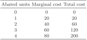
In [5] they consider an industry consisting of 5 firms (n= 5) with a default profitΠ0
= 200 ECU (Experimental Currency Unit, which is then converted into Euros at a given exchange rate, known to the subjects at the beginning of the experiment), an optimal subsidy ofs= 50 and a discrete abatement cost schedule presented in table 1. Abatement schedule and marginal damage imply a socially optimal abatement level ofa∗= 2 for anyi= 1, ...,5, leading
[image:4.595.134.281.298.366.2]to an optimal aggregate abatement level ofA∗= 10.
Table 1 Abatement cost schedule Abated units Marginal cost Total cost
0 0 0
1 20 20
2 40 60
3 60 120
4 80 200
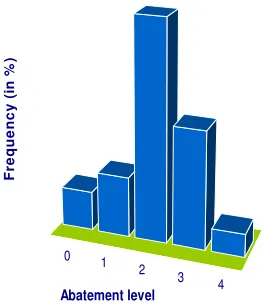
The mechanism was administered as a non-cooperative game and was re-peated over 20 periods. In total 8 sessions with 5 subjects each were con-ducted. Figure 1 illustrates the aggregate results obtained in the experiments regarding the frequency of each possible abatement decision.
3 Genetic Algorithm
The basic philosophy in implementing our version of the GA is to be “as close as possible” to the laboratory setting described in the previous section. Therefore, the parameters of the algorithms and the implementations of its internal procedures are chosen, when possible, directly from the experimental design. Additionally, we do not intend to describe a general implementation of GA, neither mention all possible alternative implementations of its operators that can be found in the literature (See [6]). Instead, we directly illustrate what we have used to implement the experimental setting.
Our genetic algorithm is characterized by the following elements:
3
4 Simone Alfarano, Eva Camacho Cuena, and Josep Dom`enech S`oria
0 1
2 3
4
0 5 10 15 20 25 30 35 40 45 50
F
re
q
u
e
n
c
y
(
in
%
)
Abatement level
Fig. 1 Histogram of experimental subjects decisions.
• Strategy:Each chromosome in the genetic algorithm represents a possible strategy that a subject can follow, that is, the abatement level decided by the subject. It is encoded as a single gene which takes integer values between 0 and 4. This is the basic element of the GA in the evolution of the algorithm. This choice follows directly the experimental setting.
• Fitness Function:It is associated to each strategy and accounts for the actual or potential payoff that derives from the use of a given strategy. In our setting, the GA player uses as measure of fitness the profit func-tion that the experimental subjects face in the laboratory (as shown in Equation 1).
• Time window:In order to associate a fitness measure to each strategy, we compute the cumulative potential profit that a given strategy would have had if played in the pastwtime periods. This time window represents the time memory that the GA subjects use to evaluate each single strategy from its population.
• Population: Each subject is endowed with a set of P strategies. The limited size of this set bounds the sophistication of the GA subject when deciding which strategy to apply.
• Mutation: It implies that with a probabilitym one of the strategies in-cluded in the population will be randomly changed into any other strategy included in the entire set of potential strategies.
[image:5.595.202.333.122.276.2]• Learning:Typically there exists two different learning mechanisms: single population vs. multi population. Under the first one, each GA agent has a set of strategies that evolve independently of the strategies of the other agents. In a multi population approach, part of the genetic material is exchanged among the GA agents. This creates some sort of interaction or imitation among agents. Given that in the laboratory setting, total abatement was the only information provided to the subjects and that no communication among subjects was allowed, we decided to implement the leaning mechanism based on a single population approach.
The number of GA agents is N = 5, following the experimental setting. Moreover, given our limited number of possible strategies, and in order to simplify the estimation procedure, we decide not to implement the crossover operator, which is typically present in the GA (see [4]). The GA parameters we aim at estimating are population (P), time window (w) and mutation rate (m).
4 Estimation: Procedure and Results
In order to estimate the key parameters of the GA described in the previous section, we fit the distribution of strategies observed in the 8 experimental sessions (See Figure 1).
Let us define asθ= (P, w, m) the vector of the parameters to be estimated.
The optimal value ofθ is calculated by minimizing the distance between the
empirical histogram of the strategies from the experimental data (see Figure 1.) and the histogram of the GA strategies computed using 5000 Monte Carlo simulations. The optimal value is then given by the following expression:
θ∗= arg min
θ
4 X
i=0
[fexp(i)−fsim(i|θ)]
2
. (2)
wherefexp(i) is the empirical frequency of the strategyicomputed from the
histogram of experimental data, and fsim(i|θ) is the frequency of strategy
i computed from 5000 Monte Carlo simulations of the GA with parameters
θ. More precisely, given a vector of parametersθ, the GA runs 5000 times
for a 20 periods4
for each realization; then the distance between the result-ing simulated histogram of strategies and the empirical one is evaluated and minimized using a Nelder-Mead optimization algorithm. The Nelder-Mead method was proposed by [11] as an unconstrained optimization algorithm. It is commonly used when the derivatives of the objective function are not avail-able. The number of Monte Carlo repetitions has been decided taking into account the computational effort and the precision of evaluation of the
sim-4
6 Simone Alfarano, Eva Camacho Cuena, and Josep Dom`enech S`oria
ulated histogram. The optimization procedure takes around an hour, which is a reasonable time. The optimal value isθ∗= (11,10,0.36).
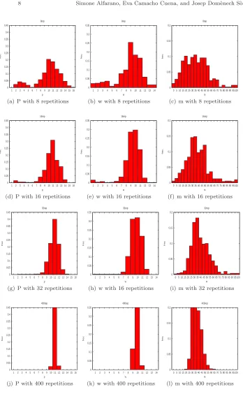
In order to evaluate the performance of the entire estimation procedure, we run a series of Monte Carlo simulations using the previously described mini-mizing procedure with artificially generated histograms as benchmark instead of the experimental data. The vector of parameters of the GA is θ∗.
Essen-tially, we re-estimate the known parameters of the GA, valuating then the
ex-post resulting distribution of the estimated θˆ. The benchmark histogram
is computed averaging over an increasing number of single simulations of 20 periods (see details in Figure 2). We have computed 500 Monte Carlo repli-cations of the re-estimation procedure for each benchmark histogram. The entire process required about 60 days of computing time, although it was parallelized in a 20-node cluster to cut the simulation time to three days.
5 Conclusions
The first important result of our computational exercise is to demonstrate that it is possible to estimate the parameters of a GA using experimental data. As it turns out, the estimation of the key-parameters of GA applied to this set of experiments gives satisfactory results, considering the small data sample available and the highly complex nature of the GA algorithm. The different parameters can be, in fact, estimated with reasonable errors, as the Monte Carlo numerical re-estimation exercise shows. We have performed the re-estimation procedure with a benchmark histogram averaged over 8, 16, 32 and 400 replications of the genetic algorithm. The case using 400 repetitions was conducted as a computational exercise to see the asymptotic properties of the estimator. From an experimental point of view, our Monte Carlo exercise shows that are enough few experimental sessions to generate a sufficiently large data set in order to reliably estimate the parameters.
Acknowledgements
Financial support from the Spanish Ministry of Science and Innovation under research project ECO2008-00510 and from Universitat Jaume I-Bancaixa under the research project P11A2009-09 is gratefully acknowledged.
References
1. Arifovic, J. (1994) Journal of Economic Dynamics and Control 18:3–28
2. Arifovic, J. (1996) Journal of Political Economy 1104:510–541
3. Aumann, R. J. (1997) games and Economic Behavior 21:2–14
4. Casari, M. (2004) Computational Economics 24:257–275
5. Camacho, E. and Requate, T. (2010) The Regulation of Non-Point Source Pollution and Risk Preferences: An Experimental Approach. Mimeo.
6. Dawid, H. (1999) Journal of Economic Dynamics and Control 23:1545–1569.
7. Duffy, J. (2006) Agent-Based Models and Human Subject Experiments. In: L. Tesfat-sion and K.L. Judd (eds) Handbooks of Computational Economics, vol. 2. Handbooks in Economic Series, Amsterdam: Elsevier
8. Hansen, L. G. (1998) Environmental and Resource Economics 12:99–112
9. Lux, T. and Schornstein, S. (2007) Journal of Mathematical Economics 44:169–196
10. Lux, T. and Hommes, C. (2008) Individual Expectations and Aggregate Behavior in Learning to Forecast Experiments Kiel Institute for the World Economy 1466
11. Nelder, J.A. and Mead, R.(1965) The Computer Journal 7:308-313
8 Simone Alfarano, Eva Camacho Cuena, and Josep Dom`enech S`oria 0 0.05 0.1 0.15 0.2 0.25 0.3 0.35 0.4 0.45
1 2 3 4 5 6 7 8 9 10 11 12 13 14 15 16
frec
p 8rep
(a) P with 8 repetitions
0 0.05 0.1 0.15 0.2 0.25 0.3 0.35
1 2 3 4 5 6 7 8 9 10 11 12 13 14
frec
w 8rep
(b) w with 8 repetitions
0 0.05 0.1 0.15 0.2
0 5 10 15 20 25 30 35 40 45 50 55 60 65 70 75 80 85 90 95 100
frec
m 8rep
(c) m with 8 repetitions
0 0.05 0.1 0.15 0.2 0.25 0.3 0.35 0.4 0.45
1 2 3 4 5 6 7 8 9 10 11 12 13 14 15 16
frec
p 16rep
(d) P with 16 repetitions
0 0.05 0.1 0.15 0.2 0.25 0.3 0.35
1 2 3 4 5 6 7 8 9 10 11 12 13 14
frec
w 16rep
(e) w with 16 repetitions
0 0.05 0.1 0.15 0.2
0 5 10 15 20 25 30 35 40 45 50 55 60 65 70 75 80 85 90 95 100
frec
m 16rep
(f) m with 16 repetitions
0 0.05 0.1 0.15 0.2 0.25 0.3 0.35 0.4 0.45
1 2 3 4 5 6 7 8 9 10 11 12 13 14 15 16
frec
p 32rep
(g) P with 32 repetitions
0 0.05 0.1 0.15 0.2 0.25 0.3 0.35
1 2 3 4 5 6 7 8 9 10 11 12 13 14
frec
w 32rep
(h) w with 16 repetitions
0 0.05 0.1 0.15 0.2
0 5 10 15 20 25 30 35 40 45 50 55 60 65 70 75 80 85 90 95 100
frec
m 32rep
(i) m with 32 repetitions
0 0.05 0.1 0.15 0.2 0.25 0.3 0.35 0.4 0.45
1 2 3 4 5 6 7 8 9 10 11 12 13 14 15 16
frec
p 400rep
(j) P with 400 repetitions
0 0.05 0.1 0.15 0.2 0.25 0.3 0.35
1 2 3 4 5 6 7 8 9 10 11 12 13 14
frec
w 400rep
(k) w with 400 repetitions
0 0.05 0.1 0.15 0.2
0 5 10 15 20 25 30 35 40 45 50 55 60 65 70 75 80 85 90 95 100
frec
m 400rep
(l) m with 400 repetitions
[image:9.595.109.457.77.641.2]