Munich Personal RePEc Archive
Arbitrarily Fast CRR Schemes
Leduc, Guillaume
American University of Sharjah, College of Arts and Sciences,
Department of Mathematics and Statistics
26 September 2012
Online at
https://mpra.ub.uni-muenchen.de/42094/
GUILLAUME LEDUC
Abstract. We introduce a method for the approximation of a lognor-mal stock price process by a Cox, Ross and Rubinstein (CRR) type of binomial scheme, which allows to reach arbitrary speed of convergence of orderO(−2), for any integer 0.
1. Introduction and Setting
Let be the standard parameters in the Black-Scholes model, and consider a European call option with strike , with expressed in the form =0 exp( ) for some real number, where0 is the spot price
of the underlying asset. Also let ©()ª∈N denote risk neutral binomial
schemes such that at every positive time in N the random walk ()
has a probability () of jumping from its current state () to the state ()(), and a probability1−()of jumping to the state()(). Risk neutral binomial schemes are of the CRR type if() = exp(q+())
and () = exp(−
q
+()
), for some bounded real valued function
. Such schemes are also calledflexible CRR binomial schemes.
Analyzing the convergence behavior of binomial schemes to calculate op-tion prices has been a popular topic, in particular for theEuropean, Amer-ican, Continuously Paying, Lookback, Digital, Game, and Barrier option types. In the case of European options approximated by CRR-type bino-mial schemes, let us mention –among others– [6], [2], [3], [1], and [5]. Let () :=( ) be the price of a European option with payoffunder the CRR-type scheme and let 0 := 0() be the price of the same option in
the Black-Scholes model. Considering a special case offlexible CRR scheme, Walsh [6] obtained an explicit formula2() :=2( )relating()and
0:
( ) =0() +
2( )
+O(−
3 2)
Date: October 2012.
1991Mathematics Subject Classification. 91B24, 91G20, 60J20 JEL Classif.: G13.
2 GUILLAUME LEDUC
Considering call options in [2] and digital options in [3], Diener and Diener showed how coefficients () can be explicitly calculated such that
(1.1) () =0+ 0
X
=2
()−
2 +O(−
0+1 2 )
Chang and Palmer [1] showed how one can choose:=() in such a way that, for European Call and digital options,
() =0+
m0
+(
−1)
Korn and Müller [5] showed how to choose:=()in order to minimizem0
in absolute value. In the cases where m0 = 0, this provides an acceleration
of the convergence to order (−1). Given any integer 2, we show in this paper how:=()can be chosen to obtain
() =0+O(−
2)
Such rate of convergence had been obtained for special binomial trees in Joshi [4] for odd, and Xiao [7] extended the argument to even. These
special binomial trees differ from the classical flexible CRR trees among other things by the fact that exactly half of the values taken by () are above the strike. Most of the commonly used binomial scheme are flexible CRR schemes. The method proposed in this paper is not only an alternative to the Joshi’s trees, but it also shows how arbitrarily fast convergence can be achieved in a quite straightforward manner for classical flexible CRR schemes, simply by choosing the parameter appropriately. Furthermore, our method has the advantage to immediately extend, with nothing but trivial modifications, the digital options in [3], and in fact, to virtually any situation where an error formula of the form (1.1) exists. For the sake of simplicity we restrict our attention to flexible CRR schemes and to call options in the setting of [2], described below.
Let 0 ≥ 2 be an integer, and let 1 = and →− = (1 2 0).
Consider binomial schemes of the form
u(−→) = exp
Ã
r
+2
2 + 0 X =3 2 r !
d(−→) = exp
Ã
−
r
+2
2 + 0 X =3 2 r !
p(−→) = exp(
)−d(
− →
and write
a(−→) =
ln³0´−ln³d( −→)´ ln³u( −→)´−ln³d( −→)´
= 2
µ
¶−1
−2
2 −
2
µ
¶−1 2 − 0 X =3 r
−3
(−→) = ³a( −→)´ Diener and Diener [2] showed that
(1.2) (−→) =0+ 0
X
=2
³−→
(−→)´−2 +O
³
−0+12
´
where, for= 2 0,
³−→
´= exp(−(−2 +
2+ 2)2
82 )0P(
− → )
and P is a multivariate polynomial in (2 ) (together with the
parameters ) which is of degree one in . Moreover, the error O(−0+12 ) is uniform in (2
0) ∈ [−LL]
0−1, for any real number
L ≥ 0. It is sometimes convenient to write P(2 ) := P(−→ )
and we use a similar convention for and the’s.
Note that, specializing to0 = 3,2 and 3 can be written as
2(2 ) =−
1 96
√
2 exp(−(−2 +822+2)2)0 √
√
P2(2 )
3(2 3 ) =−
1 3
√
2 exp(−(−2 +822+2)2)0 √
P3(2 3 ) where
P2(2 ) =42 − 32222 + 1222 + 4222
+ 8 22 + 12 2 − 96 2 + 242242
+ 96 22 − 16 222
P3(2 3 ) =−4 3 + 4 3 + 62 − 3
+ 2 + 3 22 3− 2 − 23
−6 2
2. The Acceleration Method
Given 0, and , we describe in this section a method allowing to map
the parameters (()2 ()0 ) =: −→ of the random walk () into the
coefficients (−→ ( −→)) of −
4 GUILLAUME LEDUC
remains bounded and that, for every , (−→ ( −→)) = 0, for =
2 0. As a result, (1.2) reduces to ( −→) =0+O(− 0+1
2 ), and a
convergence of order O(−0+12 ) is achieved.
First, we consider the coefficient 2(2 ). In order for it to vanish, one
must haveP2(2 ) vanishing. This is a quadratic equation in2, yielding
2=
8 + 4 ±p() 12 2
where
()= −822(−1)2−642−72 2+ 576 2(1−) We choose (arbitrarily) the "+" solution and define the function
2()= 8 + 4 +
p
() 12 2
Now in order to haveP3(2 3 ) vanishing, it suffices have
3 = −
2(2−1) (−1) (−1) 322−(2 +)
and we define the function
3()= −2(2−1) (−1) (−1) 32()2−(2 +)
Continuing this way, that is isolatingin the equationP(2 ) = 0,
and substitutingby (), for= 2 −1, one defines functions (),
for= 2 0. This is easily done sinceP is linear in. By induction, it
is clear, that all ()have the form
() =
³
p()´
³
p()´
for some polynomials( )and( ). Assume that()0on some subinterval of(01). Obviously,(
p
()) = 0, only for finitely many values of in . Staying in between two such points, one can pick a close bounded subinterval0of such that the functions ()are all real-valued
and bounded on0, for= 2 0.
Recall that
(2.1) ( 2 0) =
Ã
2 −
22 −
2√
√
−
0
X
=3
r
−3!
and define the function
( )= ³ 2() 0()´ If, for all sufficiently large, we can solve the equation
for ∈0, then, setting
() = ()
for= 2 , and defining
− →
= ³ ()2 ()0 ´
one gets=(−→)and (→− (−→)) = 0, for = 2 0, so that
( −→) =0+O(− 0 +1
2 )
as wanted.
A glimpse at (2.1) reveals that solving=( ), is the same as solving
˚( )∈N, where
˚( )= 2 −
2()2−
2√
√
−
0
X
=3
()
r
−3
−
Note that for sufficiently large values of ,˚( ) behaves (as a function
of ∈ 0) as (2()2 −)
√
(2√), and it is obvious that, as tends to infinity, the number of solutions to˚( ) ∈ N tends to
infinity. It is trivial tofind such solutions numerically in a logarithmic time by exploiting the mean value theorem.
Note that −→ exists if and only if there is a subinterval 1 of (01) on
which () is real valued, that is for which()0. Clearly this is the
case if () has some roots, which occurs when
(2.2) 722−8 2+ 162 −822−64 0
This condition is at least satisfied for small values of . In the important case of= 1(i.e. the strike is chosen such that the stock is at the money) then condition (2.2) is valid for2 12 which should always be satisfied
in practical applications.
3. Numerical Illustration
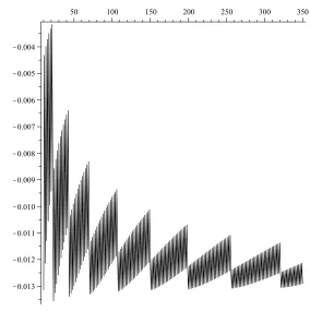
To demonstrate the performance of our acceleration method we consid-ered the case of 0 = 4 Given a strike –recall incidentally that =
0 exp( )– we define the error() as
()= ( 2() ()3 ()4 )−0
Using = 05, = 1, = 005, 0 = 1 and = 15, we computed
the quantity 52
() which oscillates heavily, but remains bounded,
illustrating numerically that the convergence is of orderO(−52) (see Figure
1).
Acknowledgement
6 GUILLAUME LEDUC
50 100 150 200 250 300 350
[image:7.612.186.470.59.344.2]K0.013 K0.012 K0.011 K0.010 K0.009 K0.008 K0.007 K0.006 K0.005 K0.004
Figure 1. The quantity 52
()remains bounded.
References
[1] Chang, L.B. and Palmer, K., 2007.Smooth convergence in the binomial model, Finance and Stochastics11no. 1, 91—105.
[2] Diener, F. and Diener, M., 2004.Asymptotics of the price oscillations of a European call option in a tree model, Mathematicalfinance14no. 2, 271—293.
[3] Diener, F. and Diener, M., 2005.Higher-order terms for the de Moivre-Laplace theorem, Contemporary Mathematics373191—206.
[4] Joshi, M.S., 2010. Achieving higher order convergence for the prices of European op-tions in binomial trees, Mathematical Finance20no. 1, 89—103.
[5] R. Korn and S. Müller, 2012.The optimal-drift model: an accelerated binomial scheme, Finance and Stochastics, 1—26.
[6] Walsh, J.B., 2003. The rate of convergence of the binomial tree scheme, Finance and Stochastics7no. 3, 337—361.
[7] Xiao, X., 2010. Improving speed of convergence for the prices of European options in binomial trees with even numbers of steps, Applied Mathematics and Computation
216, no. 9, 2659—2670.
American University of Sharjah, P.O. Box 26666, Sharjah, United Arab Emirates