Munich Personal RePEc Archive
Menu Costs and Dynamic Duopoly
Kano, Kazuko
The University of Tokyo
14 December 2011
Online at
https://mpra.ub.uni-muenchen.de/42617/
Menu Costs and Dynamic Duopoly
Kazuko Kano†
Graduate School of Economics The University of Tokyo Hongo 7-3-1, Bunkyo-ku Tokyo 113-0033, Japan Email: kkano@e.u-tokyo.ac.jp
Current Draft: November 14, 2012
Abstract
Examining a state-dependent pricing model in the presence of menu costs and dynamic duopolistic interactions, this paper claims that the assumption regarding market structure is crucial for iden-tifying the menu costs for price changes. Prices in a dynamic duopolistic market can be more rigid than those in more competitive markets, such as a monopolistic-competition market. Therefore, the estimates of menu costs under monopolistic competition are potentially biased upward due to the price rigidity from strategic interactions between dynamic duopolistic firms. By developing and estimating a dynamic discrete-choice model with duopoly to correct for this potential bias, this paper provides empirical evidence that dynamic strategic interactions, as well as menu costs, play an important role in explaining the observed degree of price rigidity in weekly retail prices.
Key Words: Menu Costs; Dynamic Discrete Choice Game; Retail Price.
JEL Classification Number: D43, L13, L81.
†This paper is based on the third chapter of my doctoral thesis, and was previously circulated under the title “Menu
1.
Introduction
In this paper, I study a structural state-dependent pricing model with menu costs for price changes
in which brands of retail products play a dynamic game of price competition. The model provides
the claim of this paper: the estimates of menu costs identified under a maintained hypothesis of
monopolistic competition could be biased upward due to the price rigidity generated from dynamic
strategic interactions between two brands in a duopolistic market. Using scanner data collected
from a large supermarket chain in the Chicago metropolitan area, I provide empirical evidence
that not only menu costs but also dynamic strategic interactions play an important role in the
high-frequency movements of weekly retail prices after correcting for potential bias. To the best
of my knowledge, the bias in the estimates of menu costs due to dynamic strategic interactions
in a duopolistic market has not been investigated thoroughly in the literature on state-dependent
pricing.
Following past studies, this paper defines menu costs as any fixed adjustment costs a price
setter has to pay when changing its price, regardless of the magnitude and direction of a price
change. Several papers provide evidence that menu costs are empirically important in
under-standing retail price dynamics. Constructing direct measures of physical and labor costs in large
supermarket chains in the United States, L´evy, Bergen, Dutta and Venable (1997) claim that menu
costs play an important role in the price setting behavior of retail supermarkets. Estimating menu
costs as structural parameters of single-agent dynamic discrete-choice models in monopolistically
competitive markets, Slade (1998) and Aguirregabiria (1999) find that their estimates of menu
costs are positive and statistically significant. More recently, using a dynamic oligopoly
competi-tion model, Nakamura and Zerom (2010) observe that menu costs are crucial for explaining price
rigidity in the short run.
As is frequently observed in macroeconomics literature, monopolistic competition is the
most commonly adopted market structure in past studies on price rigidity.1
This hypothesis of
market structure, however, is problematic if the market under study is dominated by a small
num-ber of firms. In this case, duopolistic/oligopolistic competition may be a more appropriate market
1
The seminal paper that applies a monopolistic-competition model to aggregate price rigidity is Blanchard and
structure for studying firms’ pricing behaviors. More importantly, if duopolistic/oligopolistic
com-petition prevails in the market of investigation, the estimates of menu costs identified under the
maintained assumption of monopolistic competition may be biased due to tighter strategic
interac-tions among firms. For example, suppose that there are just two dominant firms in a market that
compete in price. Although monopolistic-competition models create a degree of strategic
comple-mentarity among firms’ prices, each firm perceives its own market power to be so small that it
recognizes the average price to be exogenous. In contrast, in a duopolistic market, firms explicitly
take into account strategic interactions. Because this would lead to a stronger degree of strategic
complementarity, firms may prefer less aggressive price competition. Due to their tighter strategic
interactions, the equilibrium price of the market may be rigid to some extent regardless of the
existence of menu costs. Within such markets with tighter strategic interactions among firms, the
working hypothesis of monopolistic competition spuriously results in the overestimation of menu
costs. This situation implies that in order to draw a precise inference on menu costs, it is essential
to properly identify the market structure of a product under investigation and allow for dynamic
duopolistic/oligopolistic interactions among the firms in the market.
Although a number of empirical papers study price rigidity using micro data, few investigate
the relationship between the price rigidity of a product and its market structure, taking into account
the effect of dynamic duopolistic/oligopolistic interactions.2
Slade (1999) estimates the thresholds
of price changes as functions of strategic variables using a reduced-form statistical model. Assuming
that firms follow a variant of the (s, S) policy, Slade observes that firms’ strategic interactions in
a dynamic oligopolistic competition model exacerbate price rigidity. This observation suggests a
potential upward bias of the estimates of menu costs, as previously discussed. In this paper, I go
beyond the reduced-form model of Slade (1999) by developing a fully-structural dynamic
discrete-choice model equipped with menu costs and dynamic duopolistic interactions. Because the effect of
dynamic duopolistic interactions on equilibrium prices is captured by the strategies of the two firms
in the model, the rigidity due to menu costs is separately inferred from that due to dynamic strategic
2
Carlton (1986), Cecchetti (1986), and Kashyap (1995) are among the empirical studies on price rigidity that
use micro data. For more recent studies, see Nakamura and Steinsson (2008) and the references cited therein. For
theoretical studies that deal with duopolistic/oligopolistic competitions in the presence of fixed adjustment costs, see
Dutta and Rustichini (1995) and Lipman and Wang (2000). Unfortunately, it is not straightforward to construct
interactions. Another important exception is Nakamura and Zerom (2010), who investigate the
sources of the incompleteness of the pass-through of wholesale prices to retail prices observed within
the coffee industry. They construct an empirical model under dynamic oligopolistic competition
among manufacturers and identify the menu costs at the wholesale level. Their estimation indicates
that though the menu costs are negligible, they are nevertheless important for explaining the price
rigidity observed in the short run. Notice that the objective of this paper is different: I examine how
an empirical inference about menu costs might be affected when the underlying market structure
is misspecified.
By examining a small product market of graham crackers, I estimate menu costs under both
monopolistic competition and dynamic duopoly. The former is the benchmark and the latter is the
minimum extension of monopolistic competition with dynamic strategic interactions. It is worth
noting that the main claim of this paper is not a theoretical consequence of dynamic-duopolistic
competition; this is because in the estimation under dynamic duopoly, there is no restriction that
would lead to price rigidity. Thus, the estimated menu costs can be either greater or smaller than
that in the monopolistic-competition model. I find that the estimates of menu costs are statistically
significant under the two market structures. The comparison between the estimation results from
the two specifications supports the main claim of this paper: the dynamic strategic interactions
between brands result in an upward bias of the estimates implied by the benchmark specification
of monopolistic competition.
The next section describes the data used for analysis. Section 3 introduces the dynamic
discrete-choice duopoly model. Section 4 describes the empirical strategy of this paper. Section 5
reports the empirical results, and Section 6 concludes.
2.
Data
The data used in this paper are weekly scanner data collected across the branch stores of Dominick’s
Finer Food (DFF, hereafter), the second largest supermarket chain in the Chicago metropolitan area
during the sample period from September 1989 to May 1997.3
The data set contains information
3
The data set is publicly available online at the website of James M. Kilts Center, Graduate School of Business,
on actual transaction prices, quantities sold, indicators of promotions (simple price reductions and
bonus-buys), and a variable called average acquisition cost (AAC, hereafter), which is a weighted
average of the wholesale prices of inventory in each store, by stores and Universal Product Codes
(barcodes).4
The products in the data set are priced on a weekly basis, which matches the sampling
frequency of the data. The fact that the prices are actual transaction ones is ideal for studying
price rigidity as the frequency and timing of price changes are the most important statistics in this
study.
I choose standard graham crackers as the product to be analyzed for three reasons. First,
only a small number of firms dominate the market. Second, across firms, there is only one
similarly-sized package (15 or 16 ounces) for the product. Third, because a box of graham crackers is a minor
product, I can avoid the possibility that pricing is affected by competition among retailers due to,
for example, a loss-leader motivation. There are four brands in this market: two national brands
(Keebler and Nabisco), one local brand (Sarelno), and one private brand (Dominick’s). The market
share of the four brands is approximately 97 percent of the total sales of standard graham crackers.
Note that DFF buys graham crackers directly from manufacturers.5
Further, note that prices are
fairly uniform across stores; in other words, DFF does not adopt zone pricing, wherein stores are
assigned to one of three categories: high-, mid-, or low-priced stores. The zone pricing strategy is
typically used for products that sell in large volumes. In contrast, zone pricing is not adopted for
products with small sales volumes such as graham crackers, probably because it is too costly for a
retailer to tailor-make the prices of such goods. These facts suggest that manufacturers’ decisions
are more likely to be reflected in retail prices, and the pass-through rate from the wholesale price
to the retail store would be large.
Figure 1 plots the shelf prices of the four brands in a representative store, displaying the
following important aspects of the data. First, the shelf prices discretely jump both upward and
downward. Second, the prices stay at the same level for a certain period of time although temporary
price reductions or “sales” are observed quite frequently. Third, the price levels vary over time for
each brand. These patterns suggest that the pricing decisions can be decomposed into a discrete
4
For details on AAC, see Peltzman(2000).
5
The data set provides a code that indicates whether DFF buys a product directly from manufacturers or through
decision—whether or not to change the price—and a continuous decision—what level of price to
set. Thus, it is important to incorporate the discrete decision into a model.
Figure 1 also reveals another important aspect of the data: the pricing patterns of the two
national brands, Keebler and Nabisco, are similar to each other, but quite different from those of
the other two brands. Observe that the prices of the two national brands move quite frequently
around the higher levels for most of the sample period, while the prices of the other two brands
move less frequently around the lower levels. Tables 1 and 2 provide further evidence to support
this claim. Table 1 reports several summary statistics of the data across brands. The fourth column
of the table shows the market shares in terms of revenue; the fifth column shows the means of the
prices in U.S. dollars per ounce; and the sixth column shows the means of the quantities sold in
ounces. Although the two national brands, Nabisco and Keebler, have very different market shares,
their price levels are similar to each other. Table 2 summarizes the descriptive statistics related
to the frequencies of price changes. The third column shows the frequencies of price changes in
percentage terms; the fourth column shows the frequencies of downward price changes; the fifth
column shows the frequencies of upward price changes; and the sixth column shows the average
number of price changes per year. It is clear that the two national brands change their prices with
similar frequencies: as high as 33 percent on average. The frequencies of downward and upward
price changes of the two national brands are also close to each other, but those of the other two
brands are, by comparison, much lower. These observations lead to an inference that Keebler and
Nabisco are engaged in a dynamic competition that can be described by similar strategies, whereas
the other brands are not.
As previously discussed, most of the downward price changes are temporary reductions,
such as sales. As sales are conducted repeatedly, some consumers may feel that these follow some
cycle. If so, taking into account such consumer behavior can impact the estimation of demand
elasticity. One way to capture such behavior is to incorporate the information about the duration
between sales. Using store-level data, Pesendorfer (2002) finds that the duration between sales is
positively correlated with quantity sold. Hendel and Nevo (2003) show that the duration between
promotions is important for deriving a reasonable inference about the relationship between sales and
stockpiling behavior. From these findings in the literature, I exploit the indicator of promotional
The data set provides an indicator of in-store promotional activity, called a bonus-buy. A
bonus-buy may be associated with an advertisement, an in-store display, or a promotion such as
“buy-one-get-one-free.” Table 3 shows the frequency and mean duration of bonus-buy by brands.
The percentage of weeks during which bonus-buy is in effect for Keebler and Nabisco are 28 and
21, respectively. The mean bonus-buy length is approximately two weeks for both brands. The
problem with using this indicator is that it may overlap the period of a price reduction, and in
such a case, if bonus-buy is included in demand estimation along with price, the bonus-buy may
absorb a part of the price variation leading to a bias in demand elasticity.6
To examine the overlap
of bonus-buy on price reduction, I decompose price into “regular” price and “sale” price. First, I
look at the price of the two products at a representative store, store 73. I define regular price as
the modal price over 5 weeks, and sale price as any price lower than the regular price. Out of the
763 weeks of observations, sale price is seen in 243 weeks. Out of these 243 weeks, bonus-buy is in
effect for 177 weeks. In addition, bonus-buy is in effect with regular pricing for 21 weeks. Thus,
bonus-buy and price reduction do not necessarily overlap. Later, I examine whether this degree of
overlap biases the estimated parameter of demand elasticities.
As a common problem in scanner data, some observations are missing when no purchase
is made, when the product is out of stock, or when there are no data records.7
In particular, in
the case of graham crackers, there are approximately 20 weeks for which no record is available
for all brands in all stores. While it is possible to impute missing prices assuming no purchase
activity and using prices in previous periods, such imputation can cause spurious price rigidity.
Therefore, in this paper, I remove missing observations, including their lagged observations (i.e.,
list-wise deletion). As a result, I am left with unbalanced panel data for the two brands of 13,120
observations spread over 20 stores.8
When necessary, prices and other nominal monetary values are deflated with a constant
inflation rate.9 For the inflation rate, I use mean Consumer Price Index (CPI) for food obtained
6
The data set contains another indicator of in-store promotion: a simple price reduction. This variable is not used
in the analysis since there is no additional announcement effect on demand.
7
Other well-known scanner data such as A. C. Nielsen data also contain missing data in their original data. For
the problem arising from missing data in the Nielsen data, see Erdem, Keane, and Sun (1999).
8
The stores chosen are store 12, 18, 44, 47, 53, 54, 56, 59, 73, 74, 80, 84, 98, 107, 111, 112, 116, 122, 124, and 131.
9
The constant inflation rate stems from the assumption of the model in this paper. From September 1989 to May
from the website of the Bureau of Labor Statistics (BLS).
To solve the profit maximization problem of each brand, I need a measure of marginal
costs to produce graham crackers. I construct a measure of production costs by combining the
information from a box of graham crackers, the Input-Output table, and the Producer Price Index
(PPI). The main ingredients of graham crackers are wheat flour, whole grain wheat flour, sugar,
and oil. According to the Input-Output table, in addition to these ingredients, cardboard for
packaging, wage, and wholesale trade are major production factors in the cookies and crackers
industry. Obtaining the PPI of these items, I combine them according to the ratios shown in the
Input-Output table for the cookies and crackers industry. To derive the monetary value per unit,
the AAC from the DFF data set is used as a proxy for the wholesale price at the starting period. By
construction, the production costs explain approximately 35 percent of the price on average. The
appendix discusses the details of the costs. The constructed series is monthly and in dollars, and is
common to brands. Table 4 shows the summary statistics of the constructed costs. In particular, as
shown in the third column, the standard deviation of the constructed costs is fairly reduced when
it is deflated.
3.
Model
This section introduces the structural model of the paper. I describe only the duopoly model in this
section. The monopolistic-competition model is described in the appendix. The difference between
the two models is whether a brand takes into account the impact of its own action on the rival’s
reactions and future strategic interactions.
The model describes a dynamic competition between two brands to maximize their own
inter-temporal profits from each store. Brands set wholesale prices for each store given the strategy
of the other brand, and each store maximizes its joint profit from the products of the two brands.
The main competition is the one between two brands within each store as stores are assumed to
be local monopolists. Primary price setters are assumed to be brands while stores are allowed to
set prices discretionally to some extent.
1. At the beginning of each period, two brands of graham crackers observe the following
com-monly observable state variables: the previous demand conditions and store prices of both
brands, and a common marginal cost. In addition, each brand receives a private profitability
shock.
2. Brands simultaneously set wholesale prices for stores given the other brand’s strategy,
de-mand, and stores’ behavior. Brands also suggest the ranges of their profit-maximizing retail
prices to the stores. Wholesale prices and suggested prices are not observable to the rival
brand.
3. Demand shocks realize.
4. Observing wholesale prices, suggested ranges of retail prices, and demand shocks for the
two brands, each store sets the retail prices of the two products as a local multi-product
monopolist. If a store decides to change its shelf price following the suggestion made by a
brand, the brand pays the menu costs. Otherwise, the menu costs are paid by the store.
5. Demand conditions realize (customers come to stores) and purchases are made.
6. At the end of each period, stores and brands receive their profits.
The model maintains several important assumptions. First, the main competition in the
model is the one between brands. Previous works offer supportive evidence on the claim that the
main price competitors in a narrowly defined category are brands, and not stores or chains. For
example, analyzing the DFF data, Montgomery (1997) states that weekly deviations of prices from
regular prices mainly reflect manufacturers’ competitive actions. Slade (1998) assumes brands as
price setters with a passive retailer analyzing the brand competition in a saltine-cracker category.
According to telephone interviews with supermarket-chain managers, she claims that the
competi-tion important in a category is the one among brands. Stores, instead, compete by overall-offerings
of products and locations, and not on a product-by-product basis. Conducting interviews with
DFF stores, Chintagunta, Dube, and Singh (2003) confirm Slade’s claim and assume that stores
are local monopolists.10
The demand, nevertheless, may be affected by location or size of stores.
These factors are controlled by store-fixed effects in the estimation.
10
Furthermore, the data show that the timings of price changes of products across different categories of a brand
Second, shelf prices are set by each store and not by the chain. This assumption on the
pricing structure is based on data observation. The data show that pricing decisions at DFF are
centralized to a certain extent but that stores exhibit some discretional power in price setting. In
the case of graham crackers, the retail prices of a graham cracker product from one brand are
fairly uniform across stores, but the exact price levels and the timings of the price changes are not
entirely same. The correlation of the timing of price changes across stores is approximately 0.8.
In particular, sometimes, a few stores differ their prices by tiny amounts. This sort of pricing is
likely to be done on a store basis, and not on a brand or chain basis. This fact suggests that while
pricing decisions at the brand level are dominant for the price of graham crackers, stores have some
discretionary power and it is reasonable to assume that a store sets its own price.
Third, brands sell products to stores, and not to a whole chain. According to Peltzman
(2000), wholesale price is uniform across stores implying that it is the chain that negotiates with
manufacturers. Peltzman (2000), however, states that manufacturers changed their promotion
pol-icy toward DFF during the sample period to prevent stores from exploiting geographical price
differentials, thus implying that stores have a certain power in their negotiations with
manufactur-ers.
As brands behave while taking demand and stores’ behavior as given, I start the description
of my model with demand and stores’ behavior. A description of brand behavior then follows.
Suppose that stores∈ {1, ..., S} sells the products of two brandsi∈ {1,2}. For simplicity,
I assume a static linear demand function. Let qist,pist,rpist, and eist stand for the quantity, real
store price, real store price of the rival brand, and demand shock of the product of brandiat store
s in week t, respectively. The coefficients on price and rival price are allowed to be asymmetric
between brands. Defining a brand dummy variable that takes zero for brand 1 and one for brand
2 by br, the asymmetricity of the brand’s price elasticity is expressed by including a cross term,
pist×br. In the same manner, rpist×br allows asymmetric cross-price elasticity. Demand shock
eist is assumed to be mean-zero and decomposed into a store-brand specific componentξist, which
at the brand level. For example, the timing of a price change for a package of saltine clackers and graham crackers is
synchronized to some extent in a store. This observation suggests that it is ideal to model a brand as a multi-product
manufacturer, but it is infeasible in the current exercise to model a large number of choices with different brands for
may be correlated with price, and an idiosyncratic shock εd
ist: eist = ξist+εdist. I define another
variable, demand conditiondist, to include other demand shifters. The demand condition includes,
for example, an in-store promotion variable such as bonus-buy and the number of customers who
visit storesin weektas a measure of the size of potential purchase. distwill be discussed in detail
in the section on demand estimation and the construction of state variables. The demand for a
product of brandithen is
qist=dist−b0pist+b1rpist+ (b2pist+b3rpist)×br+eist, (1)
whereb0 ≥0,b1 ≥0, andb1 < b0.
Store s is a multi-product local monopolist who maximizes the joint profit generated by
the two branded products each period. Given wholesale prices (w1st, w2st) and the realization of
demand shocks (e1st, e2st), store s sets real retail prices (p1st, p2st) and puts the products on its
shelf. Part of demand conditions (d1st, d2st), such as customer count is yet to be realized. The
stores form expectations with respect to its realization. The current period profit of storesin week
tis
πst =
∑
i∈1,2
(pist−wist)qist. (2)
Solving for p1st and p2st yields the following optimal retail prices:
p∗1st=λ−
1
1 [2(b0−b2) ˜d1st+ (2b1+b3) ˜d2st+λ2w1st−b3(b0−b2)w2st] (3)
and
p∗2st =λ−
1
1 [(2b1+b3) ˜d1st+ 2b0d˜2st−b0b3w1st+λ3w2st], (4)
where ˜dist = Etdist+eist, λ1 = 4b0(b0−b2)−(2b1 +b3)2, λ2 = 2b0(b0 −b2)−b1(2b1 +b3), and
λ3 = 2b0(b0 −b2)−(b1+b3)(2b1+b3). Etdist is the conditional expectation with respect to the
demand condition, which follows an exogenous first-order Markov process.
Given the decision rule of stores described above, brands compete with respect to wholesale
prices, which are unobservable to the other brand, over infinite periods. In each period, brand i
observes the previous own and rival’s real retail prices,pist−1 and rpist−1, current real production
costs ct that are common to both brands, and the previous demand conditions dist−1 for both
demand conditions are assumed to be realized during a week. Store-level demand shockeist is not
realized yet, and brands take the same expectations with respect to its realization. At the same
time, each brand receives private information εist that affects its profitability.
Observing the state variables, (p1st−1, p2st−1, d1st−1, d2st−1, ct, εist), brands simultaneously
take their actions on real wholesale prices wist, which are drawn from a continuous support,
ex-pecting that store s follows the decision rule of equations (3) and (4). At the same time, suppose
that a brand suggests a retail price range from the L discretized bins. The suggested retail price
range contains the ex-ante optimal retail price level. Given each of the suggested price ranges,
the optimal retail behavior reflected in equation (3) and (4) implies the corresponding range of
wholesale price,wjist,j∈ {1, ..., J+ 1}, wherew1
ist is determined by pist−1. Because the suggested
price range always includes the ex-ante optimal retail price level and because the optimal retail
price perfectly reveals the underlying wholesale price through equations (3) and (4), choosing a
suggested retail price range is equivalent to choosing the corresponding wholesale price range. This
economizes the choice variable of brands and simplifies the brands’ decision problem. Below, I
for-malize the brand’s problem concentrating only on the suggested price range as the single relevant
choice variable. Both wholesale price and suggested retail price are observable only to the store
and the brand.
The offer of a wholesale price may cause a change in the nominal retail price; this incurs
menu costs. The relationship between real pricepistand nominal pricePistis given by a one-to-one
correspondence, log(pist) = log(Pist)−ρt, where ρ >0 is a constant inflation rate. I assume that
if a resulting retail price change is “large” and the change is in accordance with a store’s ex-ante
optimal retail price, the brand pays menu costs. If the price change is “small’ and not expected
ex-ante, the store pays menu costs.
I first define large and small price changes. Consider a discretization of the support of real
price into L mutually exclusive discrete elements, pist ∈ {(p1,p¯1),(p2,p¯2), ...,(pL,p¯L)}. I define a
large price change as the one across different bins: pist̸= pist−1 and Pist ̸=Pist−1. A small price
change is the one within a bin: Pist̸=Pist−1 andpist=pist−1.11 A large price change corresponds
11
To see an implication of the assumption on the data sample, I discretize the actual real prices into five segments
so that each segment is visited with approximately equal probability. Nominal price changes occur 36 percent of the
to a relatively significant price change such as the offering or terminating of a large discount while
a small one is a store-specific price change of a tiny amount.
Second, I define when and by whom menu costs are paid. Suppose that the store makes a
large retail price change. If theex-post optimal price level is the same as theex-ante optimal price
level, the brand pays menu costs: γ >0. The brand also expects that depending on the realization
of the demand shock and rival’s wholesale price, theex-post optimal retail price may deviate from
theex-ante optimal retail price level. I assume, even in this case, that the brand pays menu costs if
theex-post optimal retail price is within the suggested retail price range that contains the ex-ante
optimal retail price level. At the same time, the store may change its retail price by its discretion
reflecting changes in the retail environment captured by the demand shock. I assume that the
brand is not responsible for paying menu costs with respect to such a small price change.1213
This structure assumes that the main price setters are brands, but allows retailers to exhibit
some power to affect prices accounting for various conditions in the stores. A smaller number ofL
allows stores to use greater discretion.
Private informationεjistis drawn randomly from a set ofJ ≡L+1 alternatives: {ε1
ist, ..., εJist}.
The first element ε1
ist corresponds to the case of no price change: pist = pist−1; the second ε 2
ist,
the case of a price change to (p1,p¯1): pist ∈ (p1,p¯1) and pist ̸= pist−1; and the third ε3ist, the
case of a price change to (p2,p¯2): pist ∈(p2,p¯2) and pist ̸=pist−1, and so on. This private shock
explains the gap between the retail price predicted by the model and the observed price for each
state. An interpretation of private shock would be an unobservable idiosyncratic component of the
price adjustment costs. Under such an interpretation, the adjustment costs consist of a component
discretized bins in the space of real prices. The rest of the nominal price changes are categorized into small price
changes that do not accompany changes across the bins in the space of real prices.
12
This model does not describe menu costs paid by stores. Modeling and estimating such costs requires dynamic
models for both retailers and brands, which is beyond the scope of this paper.
13
I further assume that large price changes reflect brands’ decisions while small price changes reflect stores’ decisions.
This is an identification assumption. The suggested price range and wholesale price are both unobservable to a
researcher and the other brand, and thus, it is impossible to identify who initiated a large price change for each
observation. I impose an identification assumption that a large price change is due to the suggestion made by
brands. In addition, the structure of menu costs reduces a store’s incentive to conduct a large price change by its
common to brands, stores, and price level—menu costsγ—and an idiosyncratic component.14
Let xst = {p1st−1, p2st−1, d1st−1, d2st−1, ct, br} denote the vector stacking the
common-knowledge state variables observable to the brands, store, and a researcher. The demand conditions
and production costs follow independent stationary first-order Markov processes with transition
probability matrices independent of the actions taken by the brands. Private information, which
is observable to only brand i, εist is assumed to be i.i.d. with a known density function, g(εist),
common across actions, brands, and periods of time. The choice variable of brands, suggested price
range pist, is observable only to brand i and store s.15 When brands set their suggested prices,
each brand forms an expectation with respect to the suggested price of the other brand conditional
on the commonly observable state variables.
Under the above simplification, given the rival’s choice, the one-period profit of brandiin
storesin weekt conditional on choosing a discrete alternativej is
Πjist(xst) = (wjist−ct)Et[qist] +εjist−γI(pist̸=pist−1)I(Pist̸=Pist−1), (5)
wherewjistis the wholesale price range associated with alternative j,Etstands for the conditional
expectation operator on the realization of dist, which is conditional on the current realization of
state variable xst. The one-period profit for brand i depends on the action its rival takes given
own wholesale price. A brand maximizes its expected discounted sums of future profits by taking
into account the strategy of its rival and the evolutions of demand conditions and production costs.
The objective function of brandiin store sat period tis
E{ ∞
∑
m=t
βm−tΠis(xsm)|xst, εt}, (6)
where β ∈ (0 1) is the discount factor, and E{· | xst, εt} is the conditional expectation operator
on the payoff-relevant state variables in storesat period t. As the time horizon is infinite and the
problem has a stationary Markov structure, I assume a Markov-stationary environment. I drop the
14
This interpretation is a mixture of existing models with menu costs such as Slade (1998) and Aguirregabiria
(1999), who specify menu costs as a fixed parameter, and macroeconomic studies such as Dotsey, King, and Wolman
(1999) and Nakamura and Zerom (2010), who specify menu costs as a random shock. While I keep the term of menu
costs for the constant adjustment costs, it is reasonable that there exists an idiosyncratic shock. Sources of such
shocks may be temporary changes in information gathering and processing costs, labor costs, and display costs.
15
time and store subscript from all the variables adopting the notations ofx=xst andx′=xst+1for
any variablex. I investigate only the Markov-perfect equilibrium in which brands follow symmetric
pure-Markov strategies with imperfect information.
Let σ ={σ1, σ2} denote a set of arbitrary strategies of the two brands, where σi defines a
mapping from the state space of (x, εi) into the action space. Denote the one-period profit without
private information conditional on choosing j by πσ
i(x, j). Let Viσ(x) express the value of brand
i when both brands follow strategy σ and the state is x. Furthermore, let f(x′|x, j) represent
the transition probability of the observable state variables conditional on the action of choosing
alternative j. When private information is integrated out, the corresponding Bellman equation is
Viσ(x) =
∫
max
j∈J {π σ
i(x, j) +ε j i +β
∑
x′
f(x′|x, j)Viσ(x′)}gi(εi)dεi, (7)
where Πσi(x, j) is the profit defined by common-knowledge state variables x conditional on brand
i choosing alternative j given that the rival brand follows strategy σ2. Then, the conditional
choice probability—or the best-response probability—for brand i is to choose alternative j given
the strategy of the other brand that is associated with a set of Markov strategiesσ, can be written
as
P ri(j|x) =
∫
I{j= arg max
j∈J{π σ
i(x, j) +ε j i +β
∑
x′
f(x′|x, j)Viσ(x′)}}gi(εi)dεi. (8)
Aguirregabiria and Mira (2007) show that a Markov-perfect equilibrium, associated with
equilib-rium strategy{σ∗
1, σ∗2}is characterized as a set of probability functions{P r1(x), P r2(x)}that solve
the coupled-fixed-point problem presented by equations (7) and (8) in its probability space. The
representation in the probability space is used to describe the likelihood function for estimation.16
As noted previously, the monopolistic-competition model is described in the appendix. The
important difference between the monopolistic-competition model and the duopoly model in this
paper is that following Slade (1998) and Aguirregabiria (1999), I treat the evolution of rpist as
exogenous in the econometric model. An interpretation of this treatment would be that a brand
takes into account its rival’s price but treats the effect of its own decision through the rival’s
reaction in the future as trivial. In other words, the observed outcomes are simply those of the
static Bayesian-Nash equilibrium. In this sense, the monopolistic-competition model studied in the
16
previous papers lacks dynamic strategic interactions.17
Note that in the duopoly model, no detailed structure to introduce price rigidity due to
dynamic strategic interactions, such as collusion, is imposed. Therefore, the estimates of menu-cost
parameters under the assumption of a dynamic duopoly can be either smaller or greater than those
under the assumption of monopolistic competition. The strategy of this paper is to see whether
the data reveal this bias.
4.
Empirical strategy
This section describes the empirical implementation of the model. I first estimate demand equation.
Second, the state variables are constructed, and their transition probability matrices are estimated.
Third, wholesale price ranges are constructed. Finally, the menu costs parameter is estimated. I
describe the details below in order.
4.1. Demand estimationDemand equation (1) is common to the duopoly model and the
monopolistic-competition model. In this section, I discuss only the endogeneity problem in demand estimation,
and leave the detailed description of the estimation to the next section.
Demand error termeist is assumed to include the unobserved store-brand term that affects
demand and possibly correlates with price variables. Having included a brand dummy variable
and time dummies,ξist may include unobserved promotional activity (Nevo and Hatzitaskos 2006)
and weekly in-store valuation affected by shelf space and display (Chintagunta, Dube, and Singh
2003). To control for these endogeneities, I need an effective promotional variable or instruments
that are correlated with price but uncorrelated with the weekly store-brand demand error term.
First, I include a promotional variable, that is, a bonus-buy indicator provided by the data set.
Second, I use AAC as instrumental variables for the price. The correlation between the retail price
and AAC is 0.73 in my sample. Chintagunta, Dube, and Singh (2003) use a measure of wholesale
cost created from AAC and its lags as instruments. Having controlled for display and feature,
17
These two papers, however, feature other aspects of the models that are absent from this paper. Slade (1998)
incorporates consumer goodwill accumulated from price reductions into her model. Aguirregabiria (1999) finds a
they argue that the wholesale price, which is uniform across stores, is independent of current
store-brand demand. Nevo and Hatzitaskos (2006), who study both category and product demand over
a chain, use AAC as the instrument of price in one of their estimations.18
They note the potential
endogeneity of AAC, since regarding it as a wholesale price, it may be correlated with unobserved
promotion captured in the error term. They, however, also note that AAC does not denote the
current wholesale prices but the weighted average of past and current wholesale prices, and thus
they conclude that the problem will be less serious. I also assume that the rival and Salerno and
Dominick’s prices are endogenous, and use the corresponding AAC and their lags as instruments.
One problem in the data set is that prices show fairly small variations across stores. The
timings of price changes synchronize across stores for approximately 80 percent of the period.
This lack of cross-sectional variations in prices may be problematic in estimating pricing behaviors
because using the observations from all the stores results in spuriously small standard errors of the
estimates of menu costs without much difference in their values.19
Therefore, in the exercise below,
I provide the results from the five stores that have the fewest missing observations. The number of
observations is now 3694.
4.2. State variables From the estimated demand equation, I construct demand condition dist,
computed from the estimated coefficients on cc, sdp, bonus,duration, and duration bonus 2, store
and time dummy variables, outlier, and a constant in demand equation. The state variables consist
ofxi={p1, p2, d1, d2, c, br} in the duopoly model andxsi ={p, rp, d, rd, c, br}in the
monopolistic-competition model.
State space is discretized according to a uniform grid in the space of the empirical probability
distribution of each variable. I apply the same state space to all the price variables: p1 and p2 for
the duopoly model andpandrpfor the monopolistic-competition model. In addition,d1andd2are
also discretized so that they have the same support. This is to ensure that the estimation results do
not depend on the difference in state space construction. Therefore, the potential difference in the
estimates of menu costs parameterγ between the duopoly model and the monopolistic-competition
model is solely due to the specification regarding the interactions between the brands.
18
The corresponding estimation result is shown in their appendix. They use the result from OLS to derive their
main result.
19
The transition probabilities of the demand condition and rival price are estimated following
the method by Tauchen (1986). This method generates more smooth transition processes than
the alternative method such as counting the number of the samples that fall into each cell of the
discretized state space. To evaluate the representative value in each cell of state space, I use the
middle point of the range of each cell.
4.3. Wholesale price As described in the model, a suggested price range corresponds to a
dis-cretized bin of observed retail price. In the empirical implementation, the suggested price ranges
are evaluated at their middle values. The corresponding wholesale price range is backed out, thereby
exploiting the optimal retail behavior.20
Solving equations (3) and (4) forw1st and w2st, wholesale price range wist is expressed as
a function of suggested pricepist as follows:
w1st = [λ2λ3+b0b23(b0−b2)]−1{λ1λ3p1st+b3(b0−b2)λ1p2st (9)
−(b0−b2)[2λ3+ (2b1+b3)b3] ˜d1st−[(2b1+b3)λ3+ 2b0b3(b0−b2)] ˜d2st}
and
w2st = [λ2λ3+b0b23(b0−b2)]−1{λ1λ2p2st+b3b0λ1p1st (10)
−[2λ2−(2b1+b3)b3]b0d˜2st−[(2b1+b3)λ2−2b0b3(b0−b2)] ˜d1st}.
Given the derived wholesale price range evaluated at its mid-value, the profit is evaluated at its
middle value as well.
4.4. Estimation of menu costs To estimate menu costs parameter γ, I exploit the nested
pseudo-likelihood (NPL) estimator developed by Aguirregabiria and Mira (2002, 2007). The advantage of
using the NPL estimator over a full-solution method is computational because I do not need to
solve a dynamic-programming problem for each iteration of the maximum-likelihood estimation of
the structural parameters of the model. Moreover, the method is useful in the current application
20
Using AAC is another way to measure the wholesale price. However, I do not directly exploit this variable since
(1) AAC need not be the same as the wholesale price if stores hold inventory, and (2) the literature does not agree
with the validity of this variable as a measure of wholesale price (Peltzman 2000). The first problem is more serious
since it allows me to estimate all the parameters in demand equation and the transition process
separately from the dynamic one, which is a menu-cost parameter in this paper. The value function
is recovered from data by exploiting the infinite-horizon Markov-stationary structure of the model.
I leave the details of the estimation procedure to the appendix.
5.
Empirical results
This section describes the empirical implementation and results of this paper. The demand equation
and the transition processes of exogenous state variables are estimated separately from the menu
costs parameter. I first describe the estimation results of demand equation; second, I state the
discretization of state variables; third, I state the construction of wholesale price; fourth, I report
the results of the estimated menu costs; and finally, I report the results of the simulation exercise
to examine the property of price rigidities implied by the estimated results and the model in this
paper.
5.1. Demand estimation results Table 5 shows the results of the demand estimations. I provide
the results of 7 specifications: 3 OLS and 4 IV estimations. In all the specifications, the
depen-dent variable is the quantity sold standardized by 10 oz. The independepen-dent variables common to
all the specifications are own price (price), rival price (rp), the weighted average of the prices of
non-national brands (Dominick’s and Sarelno) with weight being the total quantity sold in the
sample period (sdp), a brand dummy variable that takes one for Nabisco and zero for Keebler
(br), the customer count (cc), the store dummy variables, the time dummies for month and year,
and the dummy variable to control for outliers.21
The customer count, which is the average
num-ber of customers per day who visit the corresponding store within a week, is used to control for
the time-varying size of potential purchasers.22
The independent variables appearing in some of
the specifications are a cross term of p and br, a cross-term of rp and br, a dummy variable of
bonus-buys, the duration since the end of the last bonus-buy, and the duration within a period of
consecutive bonus-buys. All of the monetary variables are per 10 oz. and deflated by the CPI of
food in the U.S.
21
The dummy variable to control for outliers takes one when the quantity sold exceeds 5000 oz. Such events occur
2.84 percent of the times.
22
The first column shows the names of the variables. The second to the last columns show
the results of the different specifications. OLS 1 includes the following variables: price, rp, sdp,
cc, br, and constant. The store-fixed effects, time dummies, and a dummy variable to control for
outliers are also included but their coefficients are not shown. The signs of the coefficients are as
expected. The own demand elasticity evaluated at mean is -2.8. The own elasticities evaluated at
brand-specific means are -4.34 for Keebler and -2.04 for Nabisco. Elasticity, which is calculated as
∂qist ∂pist/
¯
qi
¯
pi, where ¯qi and ¯pi are the means of price and quantity of brandi, respectively, is greater for
Keebler because q¯i
¯
pi is much smaller for Keebler. The cross-elasticities are calculated as ∂qist ∂p−ist/
¯
qi
¯
p−i,
where i ∈ {1,2} and −i ∈ {2,1}. The cross-price elasticity of Keebler’s demand with respect to
Nabisco’s price is 0.64 while that of Nabisco with respect to Keebler’s price is 0.34. The fourth to
the fifth columns (OLS2) show the estimated coefficients of the specification allowing asymmetric
coefficients on own price and rival price across brands. Although the coefficients on asymmetricity
are statistically significant, the brand-specific elasticities are similar to those calculated in OLS1.
Specification OLS3 includes the following variables: bonus, which is the dummy variable
that takes one when a bonus-buy takes place and zero otherwise; bonus duration, which is the
number of weeks elapsed since the end of the last bonus-buy; and bonus duration 2, which is the
number of weeks elapsed since the beginning of the bonus-buy.23
. The coefficient on bonus shows
a positive effect, as expected. The coefficient on bonus duration is negative but not statistically
significant. Sometimes, a bonus-buy takes place for consecutive multiple periods. If most consumers
buy products during the first week of the bonus-buy, the demand for the second week may decline.
To capture such dynamics, I include the variable bonus duration 2. This variable takes one at the
second week of the bonus-buy, two at the third week, and so on. The estimated coefficient on
bonus duration 2 is negative showing that continuing the bonus-buy does not increase demand as
much as in the first week. Importantly, in OLS3, the estimated coefficients on price and the other
price variables are not significantly affected by including the variables of bonus-buy. The estimated
coefficient on price is slightly lower than that of OLS2, but bonus does not significantly absorb
the price variation. This is expected because bonus-buy is not necessarily associated with price
reduction. The estimated elasticities for both brands evaluated at the brand-specific means are
-3.99 and -2.37. The cross-price elasticities are 0.92 for Keebler’s demand and 0.22 for Nabisco’s.
23
Columns eight through last display the results of the IV estimations. IV1 shows the
esti-mated values of coefficients with AAC, lagged AAC, rival AAC, lagged rival AAC, and the AAC of
Salerno and Dominick’s as instruments treating price,rp, andsdp as endogenous variables.
Com-pared to OLS1, the size of own price coefficient increases in absolute value. IV2 includesbr ×price
and br × rp with additional instruments of the cross-term of AAC and br, and the cross-term of
rival price and br. While the sizes of own and rival price coefficients do not change much between
IV1 and IV2, the coefficient on br × price is now insignificant. Allowing asymmetry in the
coeffi-cients on rival price, the coefficient on rpincreases while its magnitude is almost same as that on
rp×br. IV3 includes bonus,duration, andbonus duration 2, which are assumed to be exogenous.
The properties of the estimated coefficients are similar to those in OLS3 except that the cross term
on own price is insignificant. In addition, the signs of the cross-price elasticities of Nabisco in IV2
and IV3 are not right, though their values are very small. IV4 treats the bonus-related variables
as endogenous. The mean-elasticities are approximately -3.4, and the brand-specific elasticities are
approximately -5.3 for Keebler and -2.3 for Nabisco. The cross-price elasticity of Keebler’s demand
is 1.56 while that of Nabisco is 0.06, showing a strong asymmetry. The result shows that Keebler’s
demand is sensitive to Nabisco’s prices while Nabisco’s demand is not. The over-identification
test by J-statistics is not rejected in all estimations, thus demonstrating empirical support for the
validity of instruments.
The results of demand estimations indicate that own-price elasticity is approximately -2.5
in OLS and -3.5 in the IV estimations when using store-level AAC and its lags as instruments.
Cross-price elasticities under OLS and IV are different: asymmetry is much stronger in the IV
estimations. Although the main claim of this paper regarding the relative size of menu costs
between the monopolistic-competition model and the duopoly model will not be affected by the
size of demand elasticity, the size of the point estimate of menu costs will not be immune. I try the
estimation of menu costs using results from both OLS and IV.
5.2. State variables Table 6 shows the means and standard deviations of the state variables before
discretization. The third column reports that price has a moderate degree of variance, demand
condition has a relatively large variance, and production costs vary little. I discretize the state
1800; that is, np= 5,nd = 6,nc= 1, and nbr = 2, where np, nd, nc, and nbr are the number of
grids for price, demand condition, cost, and brand dummy, respectively. I set the lower and upper
bounds of state space to the 5 percent and 95 percent tiles of the samples. The number of grids
of each variable is relatively small compared to the recent applications of dynamic discrete choice
models.24
This size of discretization is, however, appropriate in the current application because
the range of the choice variable, real price, is small. The 10 percent quartile of real price is 2.08
per box and the 90 percent quartile is 2.46 per box. Thus, dividing it into 5 grids creates small
bins. The last variable in the vector of state variables, br, is a fixed state variable that takes one
for Nabisco (i= 2) and zero for Keebler (i= 1). In addition, the coarseness of state space does not
affect the estimated size of menu costs. Trying estimations with various sizes of state space, I find
no systematic relationship between the coarseness of state space and the estimated size of menu
costs in the following exercise.
5.3. Wholesale price Table 7 shows the mean value of derived wholesale prices and the frequency
of wholesale price changes. On average, both brands change their wholesale prices 26 percent of
time, with Keebler making changes slightly more frequently.25
5.4. Estimation of menu costs Table 8 presents the results of the structural estimation ofγfor both
the duopoly model and the monopolistic-competition model using the result of IV4 in the demand
estimation. The size of the estimate of γ is 4.53 for the monopolistic-competition model and 1.96
for the duopoly model. While the two estimates are statistically significant at the 1 percent level,
the duopoly model results in a higher likelihood, which means a better fit to the data. Estimated
γ in the duopoly model is much smaller than that in the monopolistic-competition model. From
the difference in estimatedγ between the two models, this upward bias can be inferred to be due
to the specification of the monopolistic-competition model.
The above result depends on the specification of a demand equation and a specific size of
24
For example, the size of state space in Collard-Wexler (2010) who focuses on the U.S. concrete industry is 1.4
million. In contrast, studies such as Slade (1998) and Aguirregabiria (1999), whose results are used for comparison,
use a smaller state space.
25
When recovered wholesale price exceeds retail price, I scale down the directly recovered wholesale price so that
state space. To demonstrate the robustness of the above result, I first estimate the duopoly model
by different specifications of demand equation and then by different sizes of state space. Table
9 shows the results across different specifications of demand estimation. The second to the fifth
columns show the estimated menu costs under the assumption of the duopoly model using the
results from all the specifications. Although the results using the IV estimations are slightly higher
than those using OLS, the difference among the results is small. Thus, the result is robust with
respect to which demand estimation result is employed. Second, Table 10 shows the estimates by
different levels of state space coarseness. The rows indicate the number of grids of demand condition
nd, and the columns take the number of grids of price np. For example, nd= 2 andnp= 2 means
that the price and demand condition are divided into two grids for each. This implies that the size
of state space is 32. As stated in the section on state space, there is no systematic relationship
between the size of state space and the estimated size of the menu costs. On average, the size of
menu costs is approximately 1.85, which is close to the estimate in Table 7.
Table 11 compares the results of this paper with those of previous studies. Due to the
specific structure of this model, the estimated menu costs may not be directly comparable to the
ones in the previous studies. Nevertheless, it will be valuable to examine what factor can contribute
to the differences and similarities in the results. The first row of the table shows the result of the
duopoly model. Its point estimate of the menu costs parameter, 1.96, is greater than the result
obtained by Aguirregabiria (1999), 1.45, and the result obtained by L´evy et al. (1997), 0.52, while
it is smaller than the result obtained in Slade (1998).26
It is not surprising that the estimate
of this paper is greater than the direct measure of menu costs calculated by L´evy et al. (1997),
0.52, because my estimate captures any costs associated with price changes, whereas the reported
number by L´evy et al. (1997) includes only the physical and labor costs of price changes.
The size of menu costs with respect to the percentage of revenue is 18 percent in this
paper. While this number is much greater than those reported in previous studies, it is closest
to the estimate obtained by Slade (1998), which is fairly large in the previous studies. Note that
26
The result of Aguirregabiria (1999), 1.45, is calculated from the reported values of asymmetric menu costs using
reported shares in revenue as weights from Table 6. He also reports the results of the specification with symmetric
menu costs, whose estimated results are also close to this value (for example, 1.12 in specification 2 in Table 5). Slade
(1998) does not report the estimate of menu costs as a percentage of revenue. Revenue is calculated as the weighted
Aguirregabiria (1999) estimates menu costs using various products, while Slade (1998) examines a
single product, as do I. This difference implies that menu costs might be relatively uniform across
products in retail stores, and that the large estimate of menu costs as a percentage of revenue that
this paper observes might simply reflect the small revenues generated by graham crackers.
The bottom row of Table 11 shows the estimated value of menu costs from a recent study
by Nakamura and Zerom (2010) who use a dynamic oligopolistic model. Their estimate of menu
costs as a percentage of revenue is much smaller than the one I obtain.27
One reason may be that
when they estimate menu costs at the level of wholesale markets, their menu costs may not include
an important part of price changes at retail markets, such as the costs to print and deliver price
tags. Another reason may be the difference in the specification of the market structure between
this study and theirs. As this paper assumes a duopolistic model abstracting potential strategic
interactions with the other two brands, the estimate of menu costs in this study may still be biased
upward.
Although the estimated size of menu costs in this paper is from a single product, it is
informative to compare the size of menu costs with that calibrated commonly in past studies in
macroeconomics. For example, under a general equilibrium model with monopolistic competitions
and menu costs, Blanchard and Kiyotaki (1987) calculate that menu costs amounting to 0.08 percent
of total revenue suffices to prevent firms from adjusting their prices. The subsequent studies in
macroeconomics require a size of 0.5-0.7 percent of total revenue to fit the models to selected sample
moments and to affect aggregate price dynamics (e.g., Golosov and Lucas 2007). The empirical
results from grocery stores, as studied herein, show that the estimated size of menu costs is large
enough to have significant effects on aggregate price adjustments. Therefore, I conclude that menu
costs have significant implications for price adjustment behaviors economically and statistically.
5.5. Price rigidity and state space The above estimation result has shown that not only menu costs
but also dynamic duopolistic interactions play an important role in explaining the price rigidities
observed in the data. Menu costs comprise an exogenous source for price rigidity while strategic
interactions create price rigidity endogenously. The overall price rigidity implied by the model under
27
Their estimate of the absolute magnitude of menu costs is not comparable because their menu costs are for price
particular menu costs is expressed by the equilibrium conditional choice probabilities of no price
change. To examine the properties of price rigidity due to strategic interactions, I next examine
the properties of the conditional choice probability of no price changes by conducting a simulation
exercise.
The main results of this exercise are as follows. First, overall price rigidity is stronger in
the duopoly model than in the monopolistic-competition model. Second, own-price elasticity and
cross-price elasticities are crucial in determining how price rigidity relates to own and rival prices
in state space. As strategic complementarity becomes stronger, price tends to be more rigid in
response to the higher past price levels of both brands. Third, dynamics also play an important
role for strategic complementarity to impact price rigidity. Taking into account future reactions
leads to more complex reactions to rival’s state variables, as compared to in a myopic model under
the assumption of duopolistic competition. I discuss these three results in detail below.
Figures 2(a) to 2(d) show the contour plots of the predicted choice probabilities of no price
changes in the monopolistic-competition model and the duopoly model assuming that the menu
costs are set to be 1.96, which is the result of the duopoly model in Table 7. The results are based
on the estimation using IV4 with the number of grids beingnp= 5 andnd= 6. Figure 2(a) shows
the predicted choice probabilities of no price change in Keebler in the duopoly model; Figure 2(b),
of Keebler in the monopolistic-competition model; Figure 2(c), of Nabisco in the duopoly model;
and Figure 2(d), of Nabisco in the monopolistic-competition model. The horizontal axis shows
own past price in state space, pt−1, and the vertical axis shows rpt−1. In other words, 1 on the
horizontal axis corresponds to the lowest previous price level: p1 forp
t−1, and so on.28 Thus, the
figures can tell us how price rigidity due to strategies varies over previous own price level, previous
rival price level, and previous relative price. The discrepancy between the previous prices of the
two brands is zero on a 45-degree line. The choice probabilities for the duopoly model are those
estimated in section 4.4 while those for the monopolistic-competition model are simulated. The
choice probabilities are shown on the curves of the contour plots. The darker an area, the higher
is price rigidity.29
28
The figures are drawn using contours in MATLAB. All probabilities between the discretized prices are
approxi-mated.
29
Predicted choice probabilities are constructed conditional on the demand conditions and the production costs,
The figures highlight three important aspects of the estimated conditional choice
proba-bilities. First, the difference between the monopolistic-competition model and the duopoly model
is apparent: the monopolistic-competition model predicts lower probabilities of no price changes
than the duopoly model for both brands: 0.11 vs. 0.39 for Keebler and 0.39 vs. 0.60 for Nabisco,
on average. As noted previously, the duopoly model in this paper specifies no deep theoretical
structure to generate a higher price rigidity in the presence of dynamic duopolistic interactions.
However, since the only difference between the monopolistic competition and the duopoly model is
how strategy is formed, this result suggests that price rigidity in the duopoly model is generated
from tighter interactions between the two national brands. Such a strong strategic interaction
ob-served in the duopoly model is the primary source for upward bias in the estimates of menu costs if
the underlying data-generating process is specified as the monopolistic-competition model. Second,
the table highlights the asymmetry between the two brands. Both in the monopolistic-competition
model and the duopoly model, Keebler tends to change its price more frequently than Nabisco.
This property is consistent with the observed data. Third, price rigidity is highly responsive to
own state. Price rigidity dramatically increases as own state becomes lower, and this tendency is
more strong in the duopoly model.
The question is how the strategic interactions in the duopoly model lead to more price
rigidities as compared to the monopolistic-competition model. For example, as stated in the
intro-duction, Slade (1999) suggests that price rigidities will be stronger as previous price level is higher
due to strategic complementarity. If dynamic duopolistic competition exacerbates such strategic
complementarity, it can be the source of stronger price rigidity in the duopoly model. Such
obser-vation is, however, not seen in the previous figures. To see the effect of strategic complementarity,
I examine the changes in price rigidities as the coefficient on rival price varies. The key parameters
in this exercise are the coefficients onrpand p. Therefore, I first examine how the coefficient on p
affects the degree of price rigidity.
Figures s3(a) to 3(f) show the contour plots of the predicted choice probabilities under the
different sizes of the coefficient on p. In this exercise, I keep the degree of asymmetricity between
the brands low: the coefficients on price×br,rp×br, and br are set to be 1. The menu costs are
set to be 2.0. To highlight the impact of own price coefficient, the coefficient on rp is set to be 1,
with which strategic complementarity is fairly weak. The figures on the top show the relationship
between price rigidity and state variables of prices when the coefficient on p is as large as -30,
implying a relatively high own demand elasticity on average. This value is close to the one in the
main result. With such a high demand elasticity, the brands tend to price their products at the
lower level. The relationship reverses as the own price coefficient becomes smaller. When the size
of the own price coefficient is -20, price rigidity becomes higher as own state is higher, indicating
that the brands are exploiting less elastic demand.
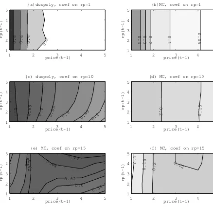
Figures 4(a) to 4(f) show the relationship between price rigidity and strategic
complemen-tarity, which is captured by the coefficient on rp. The larger size of the coefficient implies greater
strategic complementarity. These results are from an exercise similar to that in Figure 3, but now,
the coefficient on rp is changed keeping the coefficient on p at -30. The other coefficients are the
same as in Figure 3. The sizes of the coefficient on rp are 1, 10, and 15 for the top, middle,
and bottom figures. Comparing the three figures under the assumption of duopoly competition
highlights how price rigidity can vary in response to previous rival price depending on the size
of strategic complementarity. The comparison shows that first, as strategic complementarity gets
stronger, price rigidity at a higher level of own state increases. Second, price rigidities become
more responsive to rival state as strategic complementarity becomes stronger. In Figure 4(e), the
area with the highest price rigidities is the one with the highest prices, both own and rival. This is
along the intuition of Slade (1999), as discussed above. Third, as price complementarity becomes
stronger, brands are more likely to change prices as the discrepancy between own and rival prices
in state space increases. The probability of no price change is the lowest at the top-left and the
bottom-right of the figures where the discrepancy between prices is the highest. This uncovers the
strong tendency to try to catch-up with the rival in an environment with high strategic
comple-mentarities. Thus, brands become more sensitive to relative price as strategic complementarities
become greater. Finally, comparing the figures in the duopoly and the monopolistic-competition
model makes it clear that the choice probabilities of the duopoly model are more responsive to past
rival’s price. This comparison shows that strategic complementarity is more likely to lead to price
rigidity under dynamic duopolistic interactions than under the monopolistic-competition model.
The final question is how dynamics play a role in the above result. Figure 5 compares