Simulated annealing least squares twin support vector machine (SA LSTSVM) for pattern classification

Si m ul a t e d a n n e a li n g l e a s t

s q u a r e s t wi n s u p p o r t v e c t o r

m a c hi n e ( SA-L ST SV M) fo r

p a t t e r n cl a s sific a ti o n

S a r t a k h ti, JS, Afr a b a n d p ey, H a n d S a r a e e , M H

h t t p :// dx. d oi.o r g / 1 0 . 1 0 0 7 / s 0 0 5 0 0-0 1 6-2 0 6 7-4

T i t l e

Si m u l a t e d a n n e a li n g l e a s t s q u a r e s t wi n s u p p o r t v e c t o r

m a c h i n e ( SA-LST SV M) fo r p a t t e r n cl a s sific a tio n

A u t h o r s

S a r t a k h ti, JS, Afr a b a n d p ey, H a n d S a r a e e , M H

Typ e

Ar ticl e

U RL

T hi s v e r si o n is a v ail a bl e a t :

h t t p :// u sir. s alfo r d . a c . u k /i d/ e p ri n t/ 3 7 9 5 8 /

P u b l i s h e d D a t e

2 0 1 6

U S IR is a d i gi t al c oll e c ti o n of t h e r e s e a r c h o u t p u t of t h e U n iv e r si ty of S alfo r d .

W h e r e c o p y ri g h t p e r m i t s , f ull t e x t m a t e r i al h el d i n t h e r e p o si t o r y is m a d e

f r e ely a v ail a bl e o nli n e a n d c a n b e r e a d , d o w nl o a d e d a n d c o pi e d fo r n o

n-c o m m e r n-ci al p r iv a t e s t u d y o r r e s e a r n-c h p u r p o s e s . Pl e a s e n-c h e n-c k t h e m a n u s n-c ri p t

fo r a n y f u r t h e r c o p y ri g h t r e s t r i c ti o n s .

Simulated Annealing Least Squares Twin Support

Vector Machine (SA-LSTSVM) for Pattern

Classification

Javad Salimi Sartakhtia_{, Homayun Afrabandpey}a_{, Mohamad Saraee}b,∗

a_{Department of Electrical and Computer Engineering (ECE), Isfahan University of}

Technology (IUT), Esfahan, 84156-83111, IRAN

b_{School of Computing, Science and Engineering, University of Salford-Manchester,}

Manchester, United Kingdom

Abstract

LSTSVM is a relatively new version of SVM based on nonparallel twin hy-perplanes. Although, LSTSVM is an extremely efficient and fast algorithm for binary classification, its parameters depend on the nature of the problem. Problem dependent parameters make the process of tuning the algorithm with best values for parameters very difficult, which affects the accuracy of the al-gorithm. Simulated Annealing (SA) is a random search technique proposed to find the global minimum of a cost function. It works by emulating the pro-cess where a metal slowly cooled so that its structure finally “freezes”. This freezing point happens at a minimum energy configuration. The goal of this paper is to improve the accuracy of the LSTSVM algorithm by hybridizing it with simulated annealing. Our research to date suggests that this improvement on the LSTSVM is made for the first time in this paper. Experimental results on several benchmark datasets demonstrate that the accuracy of the proposed algorithm is very promising when compared to other classification methods in the literature. Also, computational time analysis of the algorithm showed the practicality of the proposed algorithm where the computational time of the algorithm falls between LSTSVM and SVM.

Keywords: Twin Support Vector Machine, Least Squares Twin Support

Vector Machine, Simulated Annealing.

1. Introduction

Support Vector Machine (SVM), first introduced by Cortes and Vapnik [1], is a classification technique based on the Structural Risk Minimization (SRM) algorithm. The algorithm rapidly became used in many classification tasks due

∗_{Corresponding Author}

to its success in recognizing handwritten characters in which it outperformed precisely trained neural networks. In addition to recognizing handwritten char-acters, SVMs performed successful classification in other applications such as: time series prediction [2], pattern classification [3], and bioinformatics [4,5]. A comprehensive tutorial on the SVM classifier algorithm has been published by Burges [6].

After the introduction of SVM in 1995, different versions of this powerful clas-sifier were advanced including the Least Squares Twin Support Vector Machine (LSTSVM), introduced in 2009 [7]. LSTSVM combines the idea behind Least Squares SVM (LSSVM) [8] and Twin SVM (TSVM) [9].

A crucial challenge in LSTSVM and all other versions of SVM is how to set their parameters with best values. LSTSVM has four parameters which are highly dependent on the nature of the problem. Therefore, finding best values for these parameters is almost impossible for user.Our current research suggests that this is the first study to find the best values for LSTSVM parameters. However, there are several methods for dominating this challenge in SVM. Huang and Wang [10] proposed a Genetic Algorithm (GA) approach for parameter optimization. They evaluated several medicine datasets using their proposed GA-based SVM. Ren and Bai [11] also presented two approaches for parameter optimization in SVM, GA-SVM and Particle Swarm Optimization (PSO) SVM. A hybrid Ant Colony Optimization (ACO) based classifier model which simultaneously opti-mizes SVM kernel parameters and selects the optimum feature subset has been proposed by Huang [12]. Salimi et al. proposed a method that hybridized SVM and Simulated Annealing (SA) [5]. Also, Lin et al. develops a simulated an-nealing approach for parameter determination and feature selection in the SVM, termed SA-SVM [13].

Simulated Annealing is an optimization algorithm which solves the problem of becoming fixed at local minima (or maxima) by allowing less optimum moves to be chosen sometimes by some probability. The method was described inde-pendently by Scott Kirkpatrick et al. in 1983 [14] and by Vlado Cerny in 1985 [15]. Simulated annealing selects a solution in each iteration by first checking if the neighbor solution is better than the current solution. If it is, the new solu-tion will be accepted uncondisolu-tionally. If however, the neighbor solusolu-tion is not better, it will be accepted based on some probability depending on how much it differs form the neighbor solution and the value of the current solution. In this paper, we have integrated Simulated Annealing with LSTSVM to identify the optimal parameters which enhance LSTSVM accuracy. Our experimental results have demonstrated that the proposed method has higher accuracies com-pared to other well-known versions of SVM. Also, for all evaluated data sets the proposed algorithm outperformed C4.5 which is a powerful algorithm in clas-sification context. Furthermore, computational time analysis showed that our proposed algorithm is faster than SVM and it is completely a practical algo-rithm for classification tasks.

Section4gives the experimental results, and finally in Section5conclusions are presented.

2. Basic Concepts

This section presents a brief review of different versions of SVM. The versions presented are the standard SVM, TSVM, and LSTSVM.

2.1. Support Vector Machine

SVM is a maximum margin classifier which means that its goal is to minimize classification error and at the same time maximize the margin between two classes. For example, given a set of training points (xi, yi), i = 1,· · ·, n each

input training data xi ∈ Rd belongs to either of two classes with labels yi ∈ −1,+1. SVM seeks a hyperplane with equationw.x+b= 0 which can satisfy the following constraints

yi(w.xi+b)≥1, ∀i. (1)

wherew is the weight vector and b is the bias term. Such a hyperplane could be obtained by solving equation2:

M inimize f(x) = kwk

2

2 (2)

subject to yi(w.xi+b)−1≥0

The geometric interpretation of this formulation is depicted in Figure1 for a toy example.

Figure 1: Geometric interpretation of SVM

2.2. Twin Support Vector Machine

In SVM only one hyperplane performs the task of partitioning samples into two groups of positive and negative classes. In 2007, Khemchandani et al. [9] proposed TSVM to use two hyperplanes in which samples are assigned to a class according to their distance from each hyperplane. The main equations of TSVM are:

xiw(1)+b(1)= 0 (3)

xiw(2)+b(2)= 0

where w(i) _{and b}(i) _{are weight vectors and bias terms of the i}th _hyperplane.

In TSVM each hyperplane is a representative of the samples of its class. This concept is geometrically depicted in Figure2for a toy example.

Figure 2: Geometric interpretations of Twin SVM

In TSVM, the two hyperplanes are non-parallel with each being closest to the samples of its own class and farthest from the samples of the opposite class [16, 17]. Assuming A and B indicate data points of class +1 and class −1, respectively, the two hyperplanes are obtained by solving (4) and (5).

M inimize 1

2(Aw

(1)_+e

1b(1))T(Aw(1)+e1b(1)) +c1eT2q (4)

w.r.t w(1), b(1)

subject to −(Bw(1)+e2b(1)) +q≥e2, q≥0

M inimize 1

2(Bw

(2)_+e

2b(2))T(Bw(2)+e2b(2)) +c2eT1q (5)

w.r.t w(2), b(2)

In these equations, q is a vector contains the slack variables, ei (i ∈ {1,2})

is a column vector of ones with arbitrary length, and c1 and c2 are penalty

parameters. Once the hyperplanes are obtained, a new data point is assigned to class +1 or class−1 depending on to which hyperplane the point is closer in terms of perpendicular distance.

In TSVM, the number of constraints in the equation of each hyperplane is equal to the number of samples in the opposite class. Therefore, if there is an equal number of samples in the two classes, the number of constraints for each hyperplane in TSVM is equal to half the number of constraints in SVM. The computational complexity of TSVM isO((l/2)3_{) [18]. It can be shown that the}

TSVM increases the speed of the algorithm by a factor of 4 compared to the traditional SVM, i.e. it is 4 times faster when compared to the SVM.

2.3. Least Squares Twin Support Vector Machine

LSTSVM [7, 19] is a binary classifier which combines the idea of LSSVM [8,20] and TSVM. LSTSVM employs “least squares of errors” to modify inequal-ity constraints in TSVM to equalinequal-ity constraints by solving a set of linear equa-tions rather than two Quadratic Programming Problems (QPPs). Experiments have shown that LSTSVM can considerably reduce the training time, while still achieving competitive classification accuracy [8, 21]. Because LSTSVM is a combination of TSVM and LSSVM, it dramatically reduces the time com-plexity of SVM. This is because LSTSVM solves equality constraints instead of inequality constraints as in LSSVM which makes the computational speed of the algorithm faster. The number of constraints in each hyperplane in LSTSVM is half of that in SVM which again results in very low computational complexity when compared to SVM. LSTSVM also has far better accuracy compared to SVM in most classification tasks.

LSTSVM finds its hyperplanes by minimizing equations (6) and (7) which are linearly solvable. By solving (6) and (7), values ofwandbfor each hyperplane are obtained according to (8) and (9).

M inimize 1

2(Aw

(1)_+eb(1)₎T_(Aw(1)_+eb(1)_{) +}c1

2q

T_{q (6)}

w.r.t w(1), b(1)

subject to (Bw(1)+eb(1)) +q=e

M inimize 1

2(Bw

(2)_+eb(2)₎T_(Bw(2)_+eb(2)_{) +}c2

2q

T_{q (7)}

w.r.t w(2), b(2)

subject to (Aw(2)+eb(2)) +q=e

w(1) b(1)

=−(FTF+ 1

c1

w(2)

b(2)

=−(ETE+ 1

c2

FTF)−1ETe (9)

where E =

A e

and F =

B e

whereas A, B, e and q are introduced in Section2.2.

3. Proposed Algorithm

LSTSVM has four parametersc1,c2, sigma1 andsigma2 which should be

set by the user wherec1andc2 represent the amount of error for each class and

sigma1andsigma2measure the impact of error on each hyperplane. These four

parameters are highly dependent on the nature of the problem which means that for different problems, they would have different optimum values. This affects the accuracy of LSTSVM and is considered as a weakness.

Genetic algorithms, analytical gradient, numerical gradient and Monte Carlo are examples of methods used to find the optimum values for the parameters. Simulated Annealing (SA) is also used to find global optimum values for param-eters. Although SA is time consuming, it achieves better accuracies compared to other methods. In this study the SA algorithm is used to find the best global values for LSTSVM parameters.

3.1. Simulated Annealing

SA is a technique to find the best solution for an optimization problem by trying random variations of the current solution. It is a generalization of a Monte Carlo method for examining equations of state and frozen states of n-body systems. Figure3shows the pseudo code of the SA heuristic.

In each step, SA considers some neighboring statesiof the current statescurrent,

and decides between moving to statesi or staying in statescurrent with some

probability. The new state (si) will be accepted if it has a better fitness

com-pared to the current state (scurrent). If however the new state has lower fitness,

it will be accepted with the probability showed in line 13 of the pseudo code. Note that the definition of “fitness” depends on the goal of the problem. These probabilistic movements ultimately lead the system to a state with almost op-timum solution.

3.2. SA-LSTSVM

This section presents the proposed SA-LSTSVM algorithm in more detail. As already stated, LSTSVM has four parameters, two for each of the hyper-planes, which depend on nature of the problem. In SA a set of states is defined where each state has a set of parameters which include c1, c2, sigma1 and

sigma2. The start state and its parameters are initiated by the user. For each

Figure 3: Pseudo Code of Simulated Annealing

difference between the parameter values of each two neighbor states, but the difference decreases as the algorithm iterates. In each iteration, a neighbor will be selected randomly. If the selected neighbor has higher accuracy than the current state, the selected neighbor will be taken and its parameters values (c

andsigma) used as new parameter values. Figure4 shows the pseudo-code of the combined algorithm.

4. Experimental Results

c= [c1, c2] andsigma= [sigma1, sigma2]

c←c0;

sigma←sigma0;

Acc= MyLSTSVM (dataset, classes, method,c0,sigma0);

cbest←c;sigmabest←sigma;Accbest←Acc;

iteration←0;iterationmax←Constant Value (e.g. ∞);

Whileiteration < iterationmax {

cnew=c−0.01 + (0.02)∗randn(1,2);

sigmanew=sigma−0.0001 + (0.0002)∗randn(1,2);

AccN ew= MyLSTSVM(dataset, classes, method, c0,sigma0);

ifexp((AccN ew−Acc)∗iteration)> rand(1,1)

{

c←cnew;sigma←sigmanew;Acc←AccN ew;

cbest←cnew;sigmabest←sigmanew;

iteration←iteration+ 1;

} }

returncbest, sigmabest, Accbest

Figure 4: Algorithm Outline: SA-LSTSVM

4.1. Small Data Sets

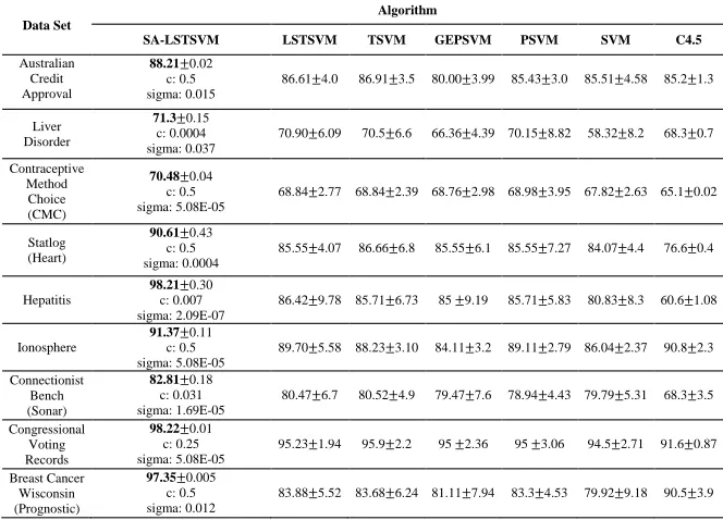
In this section, 9 standard small data sets from the UCI repository [23] were evaluated. Table1 shows some features of these data sets.

Table 1: Characteristics of the small Data Sets

Data Sets # Features # Samples Lost Data?

Australian Credit Approval 14 690 No

Liver Disorders 7 345 No

Contraceptive Method Choice (CMC) 9 1473 No

Statlog (Heart) 13 270 No

Hepatitis 19 155 Yes

Ionosphere 34 351 No

Connectionist Bench (Sonar) 60 208 No

Congressional Voting Records 16 435 Yes

Breast Cancer Wisconsin (Prognostic) 34 198 No

Table2presents the evaluation results of SA-LSTSVM and 6 other algorithms on these data sets. These algorithms are SVM, 4 different versions of SVM and a decision tree classification algorithm, C4.5 [24], which has been selected because of its good performance in classification tasks. Boldtext indicates best accuracies for each data set.

SA-Table 2: Experimental Results of SA-LSTSVM and Other Algorithms

Data Set

Algorithm

SA-LSTSVM LSTSVM TSVM GEPSVM PSVM SVM C4.5

Australian Credit Approval

88.21±0.02 c: 0.5 sigma: 0.015

86.61±4.0 86.91±3.5 80.00±3.99 85.43±3.0 85.51±4.58 85.2±1.3

Liver Disorder

71.3±0.15

c: 0.0004 sigma: 0.037

70.90±6.09 70.5±6.6 66.36±4.39 70.15±8.82 58.32±8.2 68.3±0.7

Contraceptive Method

Choice (CMC)

70.48±0.04 c: 0.5 sigma: 5.08E-05

68.84±2.77 68.84±2.39 68.76±2.98 68.98±3.95 67.82±2.63 65.1±0.02

Statlog (Heart)

90.61±0.43 c: 0.5 sigma: 0.0004

85.55±4.07 86.66±6.8 85.55±6.1 85.55±7.27 84.07±4.4 76.6±0.4

Hepatitis

98.21±0.30 c: 0.007 sigma: 2.09E-07

86.42±9.78 85.71±6.73 85 ±9.19 85.71±5.83 80.83±8.3 60.6±1.08

Ionosphere

91.37±0.11 c: 0.5 sigma: 5.08E-05

89.70±5.58 88.23±3.10 84.11±3.2 89.11±2.79 86.04±2.37 90.8±2.3

Connectionist Bench (Sonar)

82.81±0.18 c: 0.031 sigma: 1.69E-05

80.47±6.7 80.52±4.9 79.47±7.6 78.94±4.43 79.79±5.31 68.3±3.5

Congressional Voting Records

98.22±0.01 c: 0.25 sigma: 5.08E-05

95.23±1.94 95.9±2.2 95 ±2.36 95 ±3.06 94.5±2.71 91.6±0.87

Breast Cancer Wisconsin (Prognostic)

97.35±0.005 c: 0.5 sigma: 0.012

83.88±5.52 83.68±6.24 81.11±7.94 83.3±4.53 79.92±9.18 90.5±3.9

LSTSVM the best values ofcand sigmaare shown, too. Reported accuracies for TSVM, GEPSVM [25], and PSVM [26] are all extracted from [7].

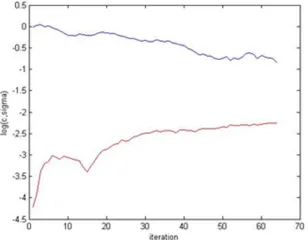
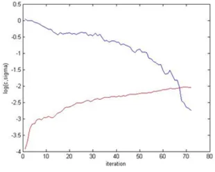
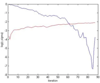
Figures 4-12 show the accuracy of the SA-LSTSVM algorithm for each of the 9 data sets for different values ofc and sigma. In some figures, the relation be-tween values of the parameters and the accuracy of SA-LSTSVM is obvious, e.g Figure 9, however for some others, e.g Figure 7 there is not an obvious relation-ship between the accuracy of SA-LSTSVM and values of the parameters. As it is mentioned before the optimum values for parameters are problem dependent. The SA algorithm is used to find the highest accuracy among continuous values ofcandsigma.

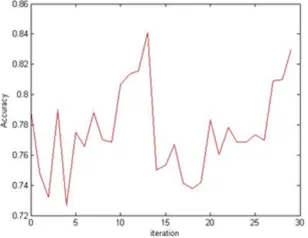
Figures 13-21 show how the values of c and sigma changed during iterations of the SA algorithm for the 9 data sets. In these figures, the blue shows the changes in the value ofc and the red curve shows how sigma changes during the iterations. As it can be seen form the figures, the way the algorithm moves toward the optimum values for parameters depends on the data set.

Figure 5: Changes in the accuracy of SA-LSTSVM for different values of c

and sigma on Australian Credit Ap-proval data set

Figure 6: Changes in the accuracy of SA-LSTSVM for different values of c

andsigmaon Liver Disorder data set

Figure 7: Changes in the accuracy of SA-LSTSVM for different values of c

andsigmaon CMC data set

Figure 8: Changes in the accuracy of SA-LSTSVM for different values of c

andsigmaon Statlog (Heart) data set

Figure 9: Changes in the accuracy of SA-LSTSVM for different values of c

andsigmaon Hepatitis data set

Figure 10: Changes in the accuracy of SA-LSTSVM for different values of c

andsigmaon Ionosphere data set

Figure 11: Changes in the accuracy of SA-LSTSVM for different values of c

andsigmaon Sonar data set

Figure 12: Changes in the accuracy of SA-LSTSVM for different values of

c and sigmaon Congressional Voting Records data set

Figure 13: Changes in the accuracy of SA-LSTSVM for different values ofcandsigma

on Breast Cancer Wisconsin data set

Figure 14: Changes ofcand sigmain SA-LSTSVM on Australian Credit Ap-proval data set

Figure 16: Changes ofcand sigmain SA-LSTSVM on CMC data set

Figure 17: Changes ofcandsigmain SA-LSTSVM on Statlog (Heart) data set

Figure 18: Changes ofcand sigmain SA-LSTSVM on Hepatitis data set

Figure 19: Changes ofcandsigmain SA-LSTSVM on Ionosphere data set

Figure 20: Changes ofcand sigmain SA-LSTSVM on Sonar data set

Figure 22: Changes ofcandsigmain SA-LSTSVM on Breast Cancer Wisconsin data set

Figure 23: Changes of the accuracy of SA-LSTSVM on Australian Credit Ap-proval data set

Figure 24: Changes of the accuracy of SA-LSTSVM on Liver Disorder data set

Figure 25: Changes of the accuracy of SA-LSTSVM on CMC data set

Figure 27: Changes of the accuracy of SA-LSTSVM on Hepatitis data set

Figure 28: Changes of the accuracy of SA-LSTSVM on Ionosphere data set

Figure 29: Changes of the accuracy of SA-LSTSVM on Sonar data set

Figure 30: Changes of the accuracy of SA-LSTSVM on Congressional Voting Records data set

4.2. Larger Data Sets

To evaluate the performance of SA-LSTSVM on larger data sets, we used David Musicant’s NDC Data Generator [27] to generate data sets with 3000, 4000, 5000, 10000, and 100000 samples and 32 features. Results of running each algorithm are shown in Table 3. The best accuracy for each data set is shown in boldface. As it is shown in the table, again SA-LSTSVM has the highest accuracies among all versions of SVM for all data sets. However, only in NDC-100k data set, C4.5 obtains a better accuracy compared to SA-LSTSVM.

Table 3: Experimental Results of SA-LSTSVM and Other Algorithms on Larger Data Sets. The∗sign shows that the algorithm did not converge in a reasonable time

4.3. Statistical Comparison of Classifiers

The above experiments showed that for all of the studied datasets, the accu-racy of SA-LSTSVM is higher than other compared algorithms. However, there still a question remains which is “Are these differences statistically significant?”. In other words, it is important to show that these algorithms are statistically dif-ferent. In [28], Demsar introduced different ways of comparing algorithms over multiple data sets. Since we have seven algorithms for comparison, we choose to use Friedman test which is a non-parametric counterpart of ANOVA. Although there are some implementations of the Friedman test in some software tools like MATLAB and KEEL [29], we chose to implement the test by ourselves in MATLAB. The Friedman test ranks the algorithms for each dataset separately in the way that the best performing algorithm getting the rank 1, the second best ranked 2 and so on. In case of ties, e.g. in CMC, Hepatitis, Congressional Voting Records, and NDC-4k, the average ranks are assigned. Table 4 shows the ranks of the classifiers for different datasets used in this paper. Numbers inside the parenthesis are the ranks of classifiers for the corresponding dataset. The final row contains the average ranks of each classifier which is computed as

Rj= _N1 P_irji, where r j

i is the rank of the j-th algorithm on the i-th dataset.

Note that since for NDC-100k two of the algorithms do not converged, we do not count this dataset in the evaluation.

Table 4: Rankings of the classifiers for each dataset

Dataset

Algorithms

SA-LSTSVM LSTSVM TSVM GEPSVM PSVM SVM C4.5

Australian Credit Approval

88.21 (1) 86.61 (3) 86.91 (2) 80.00 (7) 85.43 (5) 85.51 (4) 85.2 (6)

Liver

Disorder 71.3 (1) 70.90 (2) 70.5 (3) 66.36 (6) 70.15(4) 58.32 (7) 68.3 (5)

Contraceptive Method Choice (CMC)

70.48 (1) 68.84 (3.5) 68.84 (3.5) 68.76 (5) 68.98 (2) 67.82 (6) 65.1 (7)

Statlog

(Heart) 90.61 (1) 85.55 (4) 86.66 (2) 85.55 (4) 85.55 (4) 84.07 (6) 76.6 (7)

Hepatitis _{98.21 (1) 86.42 (2) 85.71 (3.5) 85 (5) 85.71 (3.5) 80.83 (6) 60.6 (7)}

Ionosphere _{91.37 (1) 89.70 (3) 88.23 (5) 84.11 (7) 89.11 (4) 86.04 (6) 90.8 (2)}

Connectionist Bench

(Sonar) 82.81 (1) 80.47 (3) 80.52 (2) 79.47 (5) 78.94 (6) 79.79 (4) 68.3 (7)

Congressional Voting

Records 98.22 (1) 95.23 (3) 95.9 (2) 95 (4.5) 95(4.5) 94.5 (6) 91.6 (7)

Breast Cancer Wisconsin

(Prognostic) 97.35 (1) 83.88 (3) 83.68 (4) 81.11 (6) 83.3 (5) 79.92 (7) 90.5 (2)

NDC-3k 85.16 (1) 79.24 (3) 77.73 (5) 77.20(6) 79.23 (4) 62 (7) 80 (2)

NDC-4k 84.32 (1) 79.87(3.5) 78.65 (5) 75.98 (6) 79.87 (3.5) 61.85 (7) 80.42 (2)

NDC-5k 85.40 (1) 78.93 (3) 77.49 (5) 75.43 (6) 78.01 (4) 61.72 (7) 79.52 (2)

NDC-10k 87.64 (1) 86.17(2) 85.31 (4) 84.32 (5) 85.95 (3) 61.4 (7) 82.5(6)

Average

Rank 1 2.923 3.538 5.576 4.038 6.153 4.769

Friedman statistic is compared with the statistic itself. The null-hypothesis will be rejected if the statistic is higher than the critical value.

The Friedman statistic is computed as follows:

χ2_F = 12N

k(k+ 1) 

 X

j

R2_j−k(k+ 1) 2

4 

In this equation,kandN are the total number of classifiers and the total num-ber of datasets, respectively. In our case k= 7 and N = 13. The statistic is distributed according toχ2_F withk−1 degrees of freedom, whenN and kare big enough (as a rule of thumb,N >10 andk >5) which is our case [28]. Iman and Davenport [30] showed that Friedman’sχ2_F is undesirably conservative and they proposed a better statistic as bellow.

FF =

(N−1)χ2_F N(k−1)−χ2

F

(11)

which is distributed according to the F-distribution withk−1 and (k−1)(N−1) degrees of freedom.

The computed Friedman statistic and the correspondingFF statistic for our

experiments are:

χ2_F = 12∗13 7∗8 ×

(12+ 2.9232+ 3.5382+ 5.5762+ 4.0382+ 6.1532+ 4.7692)−7∗8 2

4

= 50.3

FF =

12∗50.3

13∗6−50.3 = 21.8

With seven algorithms and 13 datasets, FF is distributed according to the F

distribution with 7−1 = 6 and (7−1)×(13−1) = 72 degrees of freedom. The critical value of F(6,72) for α= 0.05 is 2.23, so we reject the null-hypothesis which means that the algorithms are statistically different.

By rejecting the null-hypothesis we can proceed with a post-hoc test. Since we want to compare all other classifiers with our proposed SA-LSTSVM, we will use the Bonferroni-Dunn test [31]. In [28] it is explained that based on Ne-menyi test [32], the performance of two classifiers is significantly different if the corresponding average ranks differ by at least the critical difference

CD=qα

r

k(k+ 1) 6N

whereqαis the critical value.

The Bonferroni-Dunn test controls the family-wise error rate by divingαby the number of comparisons made which is k−1 in this case. The alternative way to compute the same test as it is introduced in [28] is to compute the criti-cal difference,CD, using the same equation as the Nemenyi test, but using the critical values for _(kα₋₁₎. The critical valueq0.05for seven classifiers is 2.638 and

therefore we haveCD= 2.638 q

7∗8

6∗13 = 2.235. Using this critical difference, we

• SA-LSTSVM performs significantly better that LSTSVM, since 1−2.923<

2.235

• SA-LSTSVM performs significantly better that TSVM, since 1−3.538<

2.235

• SA-LSTSVM performs significantly better that GEPSVM, since 1−5.576<

2.235

• SA-LSTSVM performs significantly better that PSVM, since 1−4.038<

2.235

• SA-LSTSVM performs significantly better that SVM, since 1−6.153 <

2.235

• SA-LSTSVM performs significantly better that C4.5, since 1−4.769 <

2.235

4.4. Computational Time Analysis

As stated in Section2.3, LSTSVM is computationally faster than SVM with a computational time better than SVM by a factor of 4. SA is a probabilistic meta heuristic algorithm which takes random walks through the problem space. This may suggest that the SA-LSTSVM algorithm may be computationally very slow. However, our computational time analysis indicates otherwise.

Table5shows the computational times in second for the SA-LSTSVM, LSTSVM and SVM algorithm for all of the data sets. For the SA-LSTSVM algorithm the maximum number of iterations considered in the experiment was 25. This number was chosen because with this value for kmax, the algorithm achieves

good accuracies for each of the different data sets. Although, we did not have any claim about the running time of the proposed SA-LSTSVM, Table5shows that the computational time of the SA-LSTSVM algorithm falls between the computational time of LSTSVM algorithm, which is the fastest version of SVM, and the standard SVM. In the table, the∗ sign shows that the computational time is extremely high and the algorithm doesn’t converge to an acceptable accuracy in a reasonable time. Although, the obtained computational times for LSTSVM are better than SA-LSTSVM and SVM, the proposed SA-LSTSVM has higher accuracies when compared to both LSTSVM and SVM for all data sets.

5. Conclusion

Table 5: Computational Time Analysis (in second) of SVM, LSTSVM and SA-LSTSVM

Data Sets \Algorithms SVM LSTSVM SA-LSTSVM

Australian Credit Approval 1.9 0.014 1.74

Liver Disorder 1.85 0.008 1.01

Contraceptive Method Choice (CMC) 3.6 0.018 0.87

Statlog (Heart) 1.58 0.013 1.11

Hepatitis 1.3 0.009 0.93

Ionosphere 1.49 0.035 0.69

Connectionist Bench (Sonar) 1.45 0.053 1.29

Congressional Voting Records 3.21 0.008 1.6

Breast Cancer Wisconsin (Prognostic) 3.73 0.028 0.8

NDC-3k 11.08 0.009 3.05

NDC-4k 22.83 0.014 7.54

NDC-5k 59.58 0.018 45.50

NDC-10k 241.68 0.026 211.56

NDC-100k ∗ 0.19 1684.82

determine the optimum parameter values for the LSTSVM algorithm. Exper-imental results on data sets with different sizes have demonstrated that the algorithm has higher accuracies compared to other well-known classification al-gorithms while its computational time is also reasonable.

References

[1] C. Cortes, V. Vapnik, Support-vector networks, Machine learning 20 (3) (1995) 273–297.

[2] J. Ruan, X. Wang, Y. Shi, Developing fast predictors for large-scale time series using fuzzy granular support vector machines, Applied Soft Comput-ing 13 (9) (2013) 3981–4000.

[3] C.-H. Wu, Y. Ken, T. Huang, Patent classification system using a new hybrid genetic algorithm support vector machine, Applied Soft Computing 10 (4) (2010) 1164 – 1177.

[4] I. Guyon, J. Weston, S. Barnhill, V. Vapnik, Gene selection for cancer clas-sification using support vector machines, Machine learning 46 (1-3) (2002) 389–422.

[5] J. S. Sartakhti, M. H. Zangooei, K. Mozafari, Hepatitis disease diagnosis using a novel hybrid method based on support vector machine and simu-lated annealing (svm-sa), Computer methods and programs in biomedicine 108 (2) (2012) 570–579.

[7] M. Arun Kumar, M. Gopal, Least squares twin support vector machines for pattern classification, Expert Systems with Applications 36 (4) (2009) 7535–7543.

[8] J. A. Suykens, J. Vandewalle, Least squares support vector machine clas-sifiers, Neural processing letters 9 (3) (1999) 293–300.

[9] R. Khemchandani, S. Chandra, et al., Twin support vector machines for pattern classification, Pattern Analysis and Machine Intelligence, IEEE Transactions on 29 (5) (2007) 905–910.

[10] C.-L. Huang, C.-J. Wang, A ga-based feature selection and parameters optimizationfor support vector machines, Expert Systems with applications 31 (2) (2006) 231–240.

[11] Y. Ren, G. Bai, Determination of optimal svm parameters by using ga/pso, Journal of Computers 5 (8) (2010) 1160–1168.

[12] C.-L. Huang, Aco-based hybrid classification system with feature subset se-lection and model parameters optimization, Neurocomputing 73 (1) (2009) 438–448.

[13] S.-W. Lin, Z.-J. Lee, S.-C. Chen, T.-Y. Tseng, Parameter determination of support vector machine and feature selection using simulated annealing approach, Applied soft computing 8 (4) (2008) 1505–1512.

[14] S. Kirkpatrick, C. D. Gelatt, M. P. Vecchi, Optimization by simulated annealing, SCIENCE 220 (4598) (1983) 671–680.

[15] V. ˇCern`y, Thermodynamical approach to the traveling salesman problem: An efficient simulation algorithm, Journal of optimization theory and ap-plications 45 (1) (1985) 41–51.

[16] S. Ding, J. Yu, B. Qi, H. Huang, An overview on twin support vector machines, Artificial Intelligence Review 42 (2) (2014) 245–252.

[17] Y.-H. Shao, C.-H. Zhang, X.-B. Wang, N.-Y. Deng, Improvements on twin support vector machines, Neural Networks, IEEE Transactions on 22 (6) (2011) 962–968.

[18] D. Tomar, S. Agarwal, Feature selection based least square twin support vector machine for diagnosis of heart disease, International Journal of Bio-Science & Bio-Technology 6 (2).

[19] Y.-H. Shao, N.-Y. Deng, Z.-M. Yang, Least squares recursive projection twin support vector machine for classification, Pattern Recognition 45 (6) (2012) 2299–2307.

[21] S. Gao, Q. Ye, N. Ye, 1-norm least squares twin support vector machines, Neurocomputing 74 (17) (2011) 3590–3597.

[22] D. Delen, G. Walker, A. Kadam, Predicting breast cancer survivability: a comparison of three data mining methods, Artificial intelligence in medicine 34 (2) (2005) 113–127.

[23] K. Bache, M. Lichman,UCI machine learning repository(2013). URLhttp://archive.ics.uci.edu/ml

[24] J. R. Quinlan, C4. 5: programs for machine learning, Vol. 1, Morgan kauf-mann, 1993.

[25] O. L. Mangasarian, E. W. Wild, Multisurface proximal support vector ma-chine classification via generalized eigenvalues, Pattern Analysis and Ma-chine Intelligence, IEEE Transactions on 28 (1) (2006) 69–74.

[26] G. Fung, O. L. Mangasarian, Proximal support vector machine classifiers, in: Proceedings of the seventh ACM SIGKDD international conference on Knowledge discovery and data mining, ACM, 2001, pp. 77–86.

[27] D. R. Musicant, NDC: normally distributed clustered datasets, www.cs.wisc.edu/dmi/svm/ndc/ (1998).

[28] J. Demˇsar, Statistical comparisons of classifiers over multiple data sets, The Journal of Machine Learning Research 7 (2006) 1–30.

[29] J. Alcal-Fdez, L. Snchez, S. Garca, M. del Jesus, S. Ventura, J. Garrell, J. Otero, C. Romero, J. Bacardit, V. Rivas, J. Fernndez, F. Herrera, Keel: a software tool to assess evolutionary algorithms for data mining problems, Soft Computing 13 (3) (2009) 307–318.

[30] R. L. Iman, J. M. Davenport, Approximations of the critical region of the fbietkan statistic, Communications in Statistics-Theory and Methods 9 (6) (1980) 571–595.

[31] O. J. Dunn, Multiple comparisons among means, Journal of the American Statistical Association 56 (293) (1961) 52–64.