MODELLING SOUND PROPAGATION AND
LOCALISATION IN ROOMS
Jonathan Sheaffer
School of Computing, Science and Engineering
University of Salford, Salford UK
Abstract 19
1 Introduction 20
1.1 Background . . . 21
1.2 Objectives and Scope . . . 25
1.3 Thesis Structure . . . 26
1.4 Contributions . . . 27
1.5 Related Publications . . . 29
2 The Physics and Perception of Spatial Sound 30 2.1 Sound Propagation . . . 31
2.1.1 The Linear Wave Equation . . . 31
2.1.2 Plane Waves . . . 32
2.1.3 Spherical Waves . . . 33
2.2 Sound in Enclosed Spaces . . . 34
2.2.1 Acoustic Impedance . . . 34
2.2.2 Boundary Conditions . . . 34
2.2.3 Reflection and Absorption . . . 35
2.2.4 The Room Impulse Response . . . 37
2.3 The Physiology of Directional Hearing . . . 39
2.3.1 The Peripheral Auditory System . . . 39
2.4.1 A Single Source in Free Field . . . 48
2.4.2 A Single Source in the Presence of Reflections . . . 53
2.4.3 Perception of Reflections and Reverberation . . . 55
3 Elements of Computational Modelling 59 3.1 Room Simulation Methods . . . 60
3.1.1 Analytical Methods . . . 60
3.1.2 Geometrical Methods . . . 60
3.1.3 Wave Methods . . . 62
3.2 Finite Difference Modelling . . . 65
3.2.1 Classical Yee Method . . . 66
3.2.2 Compact Explicit Schemes for the Wave Equation . . . 68
3.2.3 Grid Excitation . . . 71
3.2.4 Boundary Models . . . 71
3.2.5 Errors and Stability . . . 74
3.2.6 Numerical Dispersion . . . 76
3.3 Models of Sound Localisation . . . 80
3.3.1 Fundamental Modelling Concepts . . . 80
3.3.2 Applied Models of Sound Localisation . . . 83
4 Physical and Numerical Constraints in Sound Source Modelling 85 4.1 Background . . . 86
4.2 The Anatomy of Sources in Acoustics FDTD . . . 88
4.2.1 Sources in a Yee-type Method . . . 88
4.2.2 Sources in a Wave Equation Method . . . 89
4.3 Constraints in Sound Source Modelling . . . 89
4.3.1 Transduction Constraints . . . 90
4.3.2 Mechanical Constraints . . . 91
4.3.3 Numerical Constraints . . . 92
4.4 Existing Source Models . . . 93
4.4.1 Hard Sources . . . 93
4.4.3 Transparent Sources . . . 96
4.4.4 Issues with Existing Source Models . . . 97
4.5 A Cascaded Filters Approach . . . 97
4.5.1 The Pulse-Shaping Filter, Hp(z) . . . 98
4.5.2 The Mechanical Filter, Hm(z) . . . 102
4.5.3 The Injection Network . . . 103
4.5.4 A Physically Constrained Source Model . . . 104
4.5.5 Generalising Source Models . . . 107
4.6 Results . . . 109
4.6.1 Prescribed Pressure . . . 109
4.6.2 Numerical Consistency . . . 111
4.6.3 Frequency Response . . . 114
4.6.4 DC Artefacts . . . 114
4.7 Discussion . . . 118
4.8 Conclusion . . . 121
5 Practical Aspects of Room and Listener Modelling 122 5.1 The WaveCloud Project . . . 126
5.2 Oversampled Implementations on a General Purpose GPU . . . . 127
5.2.1 Algorithm Overview . . . 128
5.2.2 Thread and Memory Hierarchy . . . 129
5.2.3 Processing 3D Data Structures . . . 131
5.2.4 Algorithm Optimisation . . . 132
5.2.5 Results and Discussion . . . 133
5.3 Handling Arbitrary Room Geometries . . . 135
5.4 Modelling Binaural Receivers . . . 137
5.4.1 Listener Geometry . . . 137
5.4.2 Boundary Model . . . 137
5.4.3 Results and Discussion . . . 139
5.5 Modelling Frequency-Dependent Elements . . . 144
5.5.1 Boundary Model . . . 145
5.5.3 Discussion . . . 149
5.6 Output Visualisation . . . 151
6 An Integrated Model of Sound Localisation in Rooms Part I: Model Structure 154 6.1 Auditory Periphery . . . 155
6.1.1 Outer and Middle Ear . . . 155
6.1.2 Inner Ear . . . 157
6.2 Binaural Processor . . . 159
6.2.1 Computation of Binaural Cues . . . 159
6.2.2 Considerations for Choosing c0 . . . 161
6.2.3 Probability Density Functions . . . 162
6.3 Central Processor . . . 165
6.3.1 Cue Correlation Diagrams . . . 165
6.3.2 Across-Frequency Integration . . . 168
6.4 Discussion . . . 171
6.5 Conclusion . . . 174
7 An Integrated Model of Sound Localisation in Rooms, Part II: Results and Applications 175 7.1 A Single Source in Free Field . . . 177
7.1.1 Methodology . . . 177
7.1.2 Results . . . 178
7.1.3 Discussion . . . 180
7.2 Two Coherent Sources - Level Differences . . . 183
7.2.1 Methodology . . . 183
7.2.2 Results and Discussion . . . 184
7.3 Two Coherent Sources - Time Differences . . . 187
7.3.1 Discussion . . . 192
7.4 Effects of a Single Reflection . . . 194
7.4.1 Methodology . . . 194
7.5 Effects of Occlusion and Diffraction . . . 200
7.5.1 Methodology . . . 200
7.5.2 Results and Discussion . . . 201
7.6 Effects of Reverberation . . . 204
7.6.1 Methodology . . . 204
7.6.2 Results and Discussion . . . 205
7.7 Summary . . . 208
8 Conclusion 209 8.1 General Conclusions . . . 209
8.2 Future Challenges . . . 212
1.1 Schematic representation of a complete sound localisation model . 22
2.1 Acoustic measurement of a small (1700m3) concert hall . . . 38
2.2 Simplified schematic representation of the peripheral auditory path-way . . . 39
2.3 Cross-section of the cochlea . . . 40
2.4 Binaural Impulse Response (BIR) for a source positioned at 45◦ . 43 2.5 Illustration of the different propagation paths from a source to the two ears of a listener, resulting in interaural time and level differences. . . 44
2.6 Simplified illustration of the ascending auditory pathway . . . 45
2.7 Schematic representation of ILD and ITD processing in the audi-tory brainstem . . . 46
2.8 Geometry of a rigid sphere approximating a human head . . . 49
2.9 Left-ear HRTFs . . . 50
2.10 Frequency dependent ILDs . . . 51
2.11 Frequency dependent ITDs . . . 52
2.12 Localisation of a 150ms broadband source . . . 54
2.13 Detection thresholds of a single lateral reflection . . . 56
2.14 Detection thresholds and image-shift thresholds . . . 58
3.1 Graphical representation of a digital waveguide . . . 64
3.3 Illustration of spatial interpolation within numerical schemes for
the wave equation . . . 70
3.4 Example of different types of boundary nodes . . . 73
3.5 Dispersion error calculated for thex−y plane of a standard
recti-linear scheme . . . 78
3.6 Isotropy error for the SRL and IWB schemes . . . 79
4.1 Cascaded filter representation of source model . . . 98
4.2 Impulse response and magnitude response of different anti-dispersion
filters . . . 102
4.3 Sound pressure at the receiving position of a domain excited using
the PCS method . . . 110
4.4 Frequency response at the receiving position of a domain excited
using the PCS method . . . 111
4.5 Pressure at the receiving position for a grid excited by a hard source112
4.6 Pressure at the receiving position for a grid excited by a
differen-tiated soft source . . . 113
4.7 Pressure at the receiving position for a grid excited by a physically
constrained source . . . 113
4.8 Calculated frequency response for three different source models . . 115
4.9 Sound pressure at the receiving position for a grid excited by an
undifferentiated soft source and a physically constrained source . . 116
4.10 Source function and rate of fluid emergence at the source node, for
an undifferentiated soft source . . . 117
4.11 Source function and rate of fluid emergence at the source node, for
a physically constrained source . . . 117
5.1 General structure of the WaveCloud open software package . . . . 126
5.2 Schematic representation of a parralelised FDTD algorithm. . . . 129
5.3 Computation times of FDTD model using a GPU and a CPU. . . 134
5.4 Computer model of the Elmia concert hall . . . 135
5.5 Geometry of a KEMAR mannikin used in this study . . . 138
5.7 Calculated interaural time differences for a sphere model and a
Kemar model . . . 141
5.8 Calculated interaural level differences for a sphere model and a
Kemar model . . . 142
5.9 General structure of the multiband method. . . 144
5.10 Experimental setup for the multiband boundary model
investiga-tions. . . 146
5.11 Theoretical reflection coefficients plotted against the calculated
nu-merical reflectance . . . 147
5.12 Source directivity function as used in each of the six simulations,
corresponding to data in single octave bands. . . 149
5.13 Resulting source directivity plotted at 1/3rd octave bands, ranging
from 125−1250Hz. . . 149
5.14 Resulting source directivity plotted at 1/3rd octave bands, ranging
from 1.6−4kHz. . . 150
5.15 Volume rendering of the FDTD model of the Elmia concert hall . 152
5.16 Top-slice (Z-normal) visualisation of the FDTD model of the Elmia
concert hall . . . 152
5.17 Side-slice (Y-normal) visualisation of the FDTD model of the Elmia
concert hall . . . 153
6.1 Structure of the perceptual model . . . 155
6.2 Sound pressure at the left ear for a source at a radial distance of
1m and 30◦ to the right of a listener . . . 157
6.3 Output of the left-ear peripheral processor . . . 158
6.4 Interaural Coherence threshold as function of critical-band number 163
6.5 Probability density functions for ITD and ILD . . . 164
6.6 Cue correlation diagrams showing values of ψk˙ for a source at a radial distance of 1m and 30◦ . . . 167
6.7 Weighting function used for across-frequency integration . . . 169
6.8 Summary correlation plots for a source at a radial distance of 1m
6.9 Summary correlation plots presented over the rangeθ =±90◦ . . 170
6.10 Probability density functions for a source at 30◦ shown for the
962Hz frequency channel . . . 174
7.1 Experimental setup (individualised HRIRs) - a single source in free field . . . 177
7.2 Experimental setup (non-individualised HRIRs) - a single source in free field . . . 178
7.3 Model response as function of presented azimuth for an
individu-alised HRIR set . . . 179
7.4 Model response as function of presented azimuth for a non-individualised
HRIR set . . . 179
7.5 Model response as function of presented azimuth for a non-individualised
HRIR set, where the evaluation and corresponding integration
lim-its are confined to±90◦ . . . 180
7.6 Experiment setup for two coherent sources . . . 184
7.7 Results of modelling summing-localisation using inter-channel level
differences . . . 184
7.8 Perceived interaural cues for two sources with ICLD=10dB (right
panes) and a corresponding single source at 17◦(left panes). Upper
panes - ITD, Lower panes - ILD. . . 186
7.9 Model response as function of ICI . . . 189
7.10 Output of the binaural processor for ICIs of 4.5ms and 14ms . . . 190
7.11 Summary correlation for and ICIs of 4.5ms and 14ms . . . 190
7.12 Results of modelling summing-localisation using inter-channel time
differences . . . 191
7.13 Experimental setup for two cases of localisation at the presence of
a single reflection . . . 195
7.14 Output of binaural processor for a source at −10◦ and 1.5m away
from a listener . . . 196
7.15 Template correlation response for source at −10◦ and 1.5m away . 197
7.17 Experimental setup used in the occluded source investigations . . 201
7.18 Simulation of a sound source in free field and behind an obstacle . 202
7.19 Results for an occluded source simulation . . . 203
7.20 Experimental setup used for investigating the effects of reverberation204
7.21 Localisation error and model confidence for simulations executed
at four different source positions . . . 206
7.22 Mean localisation error and model confidence as function of
3.1 Design parameters for two commonly-used numerical schemes . . 70
4.1 Summary of existing source models in light of the constraints
dis-cussed in Section 4.3 . . . 98
4.2 Generalisation of source models using the cascaded filters approach 108
5.1 Numerical domain size and computation times for a CPU and a
GPU as function of sample rate . . . 133
5.2 Normalised impedance values and corresponding reflection factors 147
7.1 Absorption coefficients α, normalised surface impedances ξw and
˙
α Absorption coefficient
δ(·) Dirac function
γk˙ Normalised cross-correlation function at band ˙k
∇· Divergence operator
∇ Gradient operator
∇2 Laplace operator
ˆ
αk˙ Instantaneous ILD at band ˙k
ˆ
τk˙ Instantaneous ITD at band ˙k
ˆ
ck˙ Instantaneous interaural coherence at band ˙k
ξw Specific acoustic impedance (normalised)
α Damping factor
∗ Convolution operator
β Bilinear operator
λ Courant number
µ Slope of IC threshold curve
ν Surface velocity
ω Angular Frequency
ω0 Undamped angular resonance frequency
Ψ Model response azimuth
ψ Arbitrary source function
ρ0 Ambient density of air
Θ Model confidence
A( ˙k, θ0) Cue probability pattern (known azimuth)
A( ˙k, θ) Cue probability pattern (target azimuth)
ah Radius of head or sphere approximating the head
F Driving force
j Imaginary unit, √−1
K Elasticity constant
M Mass constant
Q Quality factor
q Rate of fluid emergence
R Damping constant
s Laplace variable
z Complex frequency variable
c Velocity of sound in air
CPP Cue Probability Pattern
CUDA Compute Unified Device Architecture
ERB Equivalent Rectangular Bandwidth
f Frequency
GTFB Gammatone Filter Bank
IC Inferior Colliculus
IC Interaural Coherence
ICI Inter-Click Interval
ILD Interaural Level Difference
ITD Interaural Time Difference
IWB Interpolated Wideband
JND Just Noticeable Difference
k Acoustic wavenumber
LRS Locally Reacting Surface
LSO Lateral Superior Olive
MAA Minimum Audible Angle
MSO Medial Superior Olive
PCS Physically Constrained Source
r Radial distance
SOC Superior Olivary Complex
SRL Standard Rectilinear
c0 Interaural coherence threshold
fs Sample rate
˙
k Index number of auditory filter
ˆ
n Normal component of vector
p(x, t) Acoustic pressure
Pk˙( ˆα) Probability density function for ILD
Pk˙(ˆτ) Probability density function for ITD ˆ
q Volume velocity
ˆ
r Reflection coefficient
sg Grid signal (processed source function)
sp Excitation signal
T Temporal period
u(x, t) Acoustic particle velocity
X Spatial period
xl
˙
k Output of left ear peripheral processor at band ˙k
xr
˙
k Output of right ear peripheral processor at band ˙k
Y Specific acoustic admittance
z0 Characteristic impedance of air
zw Surface impedance material
Time domain functions are written in lower case letters, e.g. p(x, t), whereas
fre-quency domain functions are written in upper case letters, e.g. P(x, ω). Discrete
signals are notated in multidimensional form. For example, an arbitrary signal u
which depends on both time and space, is notated as follows:
range 0≤f ≤0.5, where 0 is DC and 0.5 is the Nyquist frequency.
When working in a spherical coordinate system, azimuth is denoted θ,
There are many people who helped and inspired this work, both academically
and personally. First and foremost, I would like to thank my supervisor, Bruno
Fazenda, for his ongoing availability, guidance and advice, especially given the
challenging geographic circumstances behind this endeavour. Bruno is one of
the most open-minded academics I know, and has always been supportive of my
passion to explore new avenues. His ability to motivate me, see the big picture
and steer me in the right direction is very much reflected in this work.
I have had the pleasure to collaborate with some of the brightest minds in
the field of finite difference modelling. My long discussions with Maarten van
Walstijn have resulted in a fruitful collaboration which is evident in a thesis
chapter on source modelling. I would like to thank Maarten for a fantastic lesson
on academic rigour, and for always being patient and forthcoming. At earlier
stages of this work, Damian Murphy provided important insights on practical
aspects of finite difference modelling, which illuminated some fundamental issues
and resulted in a conference paper. I would also like to thank my co-supervisor,
Jamie Angus, for some interesting discussions on GPU processing, which were
very helpful in realising the WaveCloud project.
Throughout the evolution of this dissertation, I received some useful advice
from the thesis committee and I would like to thank them for taking the time
to review this work at different stages. Particularly, I would like to extend my
gratitude to the thesis examiners, Michael Vorl¨ander and Trevor Cox, for an
interesting discussion and for their useful advice. Other people who provided
Avis, Jeroen Breebaart, Alex Southern, Eldad Klaiman, Yuvi Kahana, Floyd
Toole, Nir London, John O’Hare, Hanoch Lavee, Matan Zehavi, Assaf Tal, Ohad
Dekel and my colleagues at Salford’s acoustics research centre. I apologise if I
forgot anyone.
Last but not least, I would like to thank my family without whom this journey
could not have been possible: to my children, Omer and Daphne, for occasionally
steering my attention away from acoustics, and to my parents, Zachary and Arza,
for their never-ending support. Over the past 3.5 years, my beloved spouse, Roni,
has supported me in every way possible and has always been there for me, no
Human localisation of sound in enclosed spaces is a cross-disciplinary research
topic, with important applications in auditory science, room acoustics, spatial
audio and telecommunications. By combining an accelerated model of 3D sound
propagation in rooms with a perceptual model of spatial processing, this
the-sis provides an integrated framework for studying sound localisation in enclosed
spaces on the horizontal plane, with particular emphasis on room acoustics
appli-cations. The room model is based on the finite difference time domain (FDTD)
method, which has been extended to include physically-constrained sources and
binaural receivers based on laser-scanned listener geometries. The underlying
al-gorithms have been optimised to run on parallel graphics hardware, thus allowing
for a high spatial resolution, and accordingly, a significant decrease of
numeri-cal dispersion evident in the FDTD method. The perceptual stage of the model
features a signal processing chain emulating the physiology of the auditory
pe-riphery, binaural cue selection based on interaural coherence, and a final decision
maker based on supervised learning. The entire model is shown to be capable
of imitating human sound localisation in different listening situations, including
free field conditions and at the presence of sound occlusion, diffraction and
re-flection. Results are validated against subjective data found in the literature,
and the model’s applications to the fields of room acoustics and spatial audio are
been written yet, then you
must write it.
Toni Morrison
1
Introduction
Whether we are aware of it or not, models have been an integral part of our lives
since ancient times. We build physical models to understand the operation of
mechanical systems. We look up to people who we view as role models, and draw
from their behaviour. We use fashion models as human manikins to advertise
and promote commercial products. More recently, with the availability of
com-puting technology we are also able to generate virtual models of complex physical
phenomena.
Consider, for example, a person enjoying a peaceful evening at home, when
a sudden sound of shattering glass catches his or her attention. The mechanical
motion of the breaking glass causes air particles to vibrate in a certain order and
an acoustic disturbance is generated. When this disturbance propagates, it gets
reflected off the different surfaces in the room, causing a composite sound field
to be built. At the listener’s ears, this vast amount of information is transformed
second, the listener processes this information and is able to tell, with remarkable
accuracy, where the sound is coming from. We take this process for granted. It
is an evolutionary skill essential to our survival. Yet if we wanted to model this
phenomena, how would we go about it?
1.1
Background
To cover the entire process of sound localisation in rooms, one would not only
need to model the perception of spatial sound, but also the effects of the sound
source interacting with the room itself. It is therefore acknowledged that the room
itself may play an important role in the way we localise sound. Human sound
lo-calisation is well understood in idealised environments (Gaskell, 1983; Hartmann,
1983; Rakerd and Hartmann, 1985, 1986; Hartmann and Rakerd, 1989; Blauert,
1997; Litovsky et al., 1999; Goupell et al., 2012), and such listening situations are
straightforward to measure or model. Accordingly, many sound propagation
mod-els employed in auditory research are fairly simplified, as they are only required
to account for basic acoustic phenomena, such as superposition between sources,
or reflections in a rectilinear enclosure. However, in the fields of room acoustics
and spatial audio, the effects of more advanced acoustic parameters on sound
localisation (e.g. room materials, geometry, and source directivity) present
in-teresting research questions. Thus, the ability to model sound localisation whilst
being in control of parameters in both the acoustic and psychoacoustic domains,
would be beneficial to scientists studying room acoustics, as well as to engineers
who wish to evaluate the effectiveness of their designs.
Studying room acoustics using auditory models is an emerging area of research
(Blauert et al., 2009; Blauert and Braasch, 2011; Blauert, 2013; van Dorp
Schuit-man et al., 2013), yet it appears that there is no single model that follows the
entire process, from source to brain. In this thesis, the problem of sound
locali-sation in rooms is treated as five individual processes which are integrated into a
single model, as schematically shown in Figure 1.1.
Macroscopically, the entire model can be seen as an integration of a room
Figure 1.1: Schematic representation of a complete sound localisation model and its applications.
domain and psychoacoustic domain, respectively. The room model accounts for
sound generation (source model) and propagation through the room, whereas the
perceptual model accounts for processing of the information by the peripheral
auditory system and the central nervous system. The two domains are linked by
the receiver model, whose transfer function converts the acoustic pressure field
into a binaural response. The output of the entire integrated model can be used
to evaluate the perceptual effects of changing parameters in both domains, such
as source directivity, room geometry, boundary conditions, head size and shape,
and the dynamics of the peripheral auditory system. Additionally, the different
components of the model can be used individually. The output of the room model
can be used to objectively evaluate the acoustics, either by visually inspecting the
room’s transfer function, or by extrapolating objective room parameters such as
T60, EDT,C80 and STI (Kuttruff, 2000), to name a few. Otherwise, the outputs of the receiver model can be used to create an audible rendering of the sound
source within the acoustic space, a concept known as auralisation (Kleiner et al.,
1993; Vorl¨ander, 2008).
Processes in the acoustic domain, namely the source, room and receiver, are
modelled using the Finite Difference Time Domain (FDTD) method, which has recently become more suitable for room acoustics simulation (Murphy and
Bee-son, 2007; Kowalczyk and van Walstijn, 2011). In room acoustics, the FDTD
et al., 1968; Allen and Berkley, 1979; Vorl¨ander, 1989) or other wave methods
(Ciskowski and Brebbia, 1991; Ihlenburg, 1998), and as such, one may wonder
why it has been chosen in context of this project. There are a few arguments
supporting this choice:
1. Many acoustic phenomena involving wave behaviour such as superposition
and diffraction are more difficult to handle in geometrical methods in
com-parison to FDTD. These features are especially important when studying
problems involving small rooms, and sound reproduction paradigms.
2. Being relatively new in its applications to room acoustics, the FDTD method
presents interesting avenues of research. To the author’s knowledge, FDTD
has never been used in such a wide context, and accordingly, it presents an
exciting challenge.
3. The FDTD method is straightforward to implement. As such, a customised
computer program can be generated rather than relying on third party
so-lutions. This allows the author to have full control over the entire modelling
process.
4. The FDTD method can be used to model time-variant systems, such as
walkthrough auralisation (Southern et al., 2009), moving sound sources and
even moving media (Ostashev et al., 2005). Although these features are not
directly studied in this thesis, they exemplify potential future applications
of the integrated model.
Using the FDTD method, it is now possible to model rooms with efficient
numerical schemes (Savioja and Valimaki, 2000; Kowalczyk and van Walstijn,
2011; Bilbao, 2012) and to account for frequency dependent boundaries
(Kowal-czyk and van Walstijn, 2008, 2011), diffusing boundaries (Kowal(Kowal-czyk et al., 2011)
and directional sound sources (Escolano et al., 2007). Yet, there are still some
unresolved issues which need to be addressed when employing the FDTD method
in such a broad context:
frequency response effects, with only partial solutions found in the literature
(Schneider et al., 1998a).
2. High Resolution Modelling. Similar to other wave methods, the compu-tational cost of the FDTD method is high relative to geometrical methods,
and increases dramatically with frequency. Thus, in order to accurately
model the entire audible spectrum even in a small room, one needs
exten-sive computing power.
3. Binaural Receivers. In order to interface between the acoustic domain (source and room) and psychoacoustic domain (ear and brain) or for
au-ralisation purposes, one needs to obtain binaural room responses. Insofar,
the issue of directly rendering binaural room responses using FDTD is only
partially addressed in the literature (Murphy and Beeson, 2007)
In the psychoacoustic domain, there are various approaches for modelling
the auditory periphery and prominent mechanisms in the central nervous system
which govern sound localisation. Models of the peripheral auditory system (the
middle-ear, inner-ear and associated neural transduction mechanisms) are well
established in the field of hearing science (Gigu`ere and Woodland, 1994; Meddis
and Lopez-Poveda, 2010), and can be used in a pre-processing stage of sound
lo-calisation models normally involving binaural and/or monaural processing. Some
of these models attempt to simulate neural processing mechanisms in the central
nervous system, e.g. (Goodman and Brette, 2010), some are biologically
in-spired (Jeffress, 1948; Lindemann, 1986a; Breebaart et al., 2001), whilst others
are analytically motivated (Macpherson, 1991; Faller and Merimaa, 2004b). It is
important to point out that these models aim to imitate the way humans localise
sound, unlike more general signal processing models whose goal is to perform
localisation as accurately as possible, e.g. (Valin et al., 2007; MacDonald, 2008).
It appears that models which are physiologically plausible are designed to fo-cus on the specifics of the auditory system, rather than on the general process of
sound localisation. Conversely, models which are psychoacoustically plausible do not attempt to correctly model biological processes, but to yield results which
main challenge in the psychoacoustic domain is to identify, improve and generalise
a binaural processor capable of handling acoustic settings which involve multiple
sound sources and/or sound reflections. Whilst exact emulation of the auditory
system is not necessary, such a model should at least yield psychoacoustically
plausible results.
1.2
Objectives and Scope
Drawing from these challenges, the aim of the thesis is to develop and validate a
generalised model for sound localisation in rooms, which follows the entire process
of sound generation, propagation and auditory perception. The objectives of the
thesis are:
1. To contribute to room acoustics modelling by improving the FDTD method
and enhancing its usability for simulation of realistic listening situations in
rooms.
2. To contribute to psychoacoustics modelling by developing a complete and
generalised model of sound localisation in enclosed spaces.
3. To exemplify how an integrated modelling framework, as shown in Figure
1.1, can be applied to problems in room acoustics and spatial audio.
Within the scope of this work, modelling in the psychoacoustic domain
in-volves only binaural processing, meaning that perceptual investigations are
lim-ited to localisation on the horizontal plane. Thus, the underlying assumption is
that sound sources are only presented on the same plane as the receiver. It is
em-phasised that both azimuthal and elevation reflections may contribute to binaural
localisation, and accordingly, modelling in the acoustic domain is performed in a
full 3D space.
Considering the above objectives and the defined scope of work, the modelling
framework suggested in this thesis would be particularly suited for studying the
psychoacoustic evaluation of architectural acoustics design, and with some
ad-justments, as more generalised room acoustics simulation software.
1.3
Thesis Structure
The thesis is structured as follows:
Chapter 2 provides background information on the physics and perception of
spatial sound, with focus on sound localisation in enclosed spaces. The
fundamen-tal laws of acoustics are briefly reviewed, followed by an introduction to the
phys-iology of directional hearing. These topics provide the foundations to the acoustic
and psychoacoustic models developed in the thesis. Lastly, the psychophysical
basis of sound localisation is explained, with emphasis given to interaural cues
and the perception of directional sound in rooms.
Chapter 3 provides an overview of room acoustics modelling techniques, with
emphasis on the FDTD method which is widely used in this thesis. Additionally,
the chapter provides a literature review of sound localisation methods and their
suitability to the goals of this thesis (or lack thereof).
It is noted that Chapters 2 and 3 summarise relevant information that can
be found in the literature, whereas subsequent chapters constitute the author’s
original contributions.
Chapter 4 deals with modelling sound sources for excitation of FDTD grids.
With numerical methods in mind, the fundamental physics of sound generation
and propagation are revisited, and the anatomy of sources in the FDTD method
is discussed. The merits and shortcomings of existing excitation methods is
re-viewed, and a generalised approach for modelling sources in FDTD is offered.
Finally, a novel method of exciting FDTD grids is described and compared to
existing methods.
Chapter 5 outlines the WaveCloud project, which is the computational engine
used to obtain room impulse responses in this thesis. The chapter includes a
combination of smaller contributions which together complements the practical
applications of the FDTD method. Focus is given to an accelerated
binaural receivers and to a method for modelling frequency dependent sources
and boundaries.
Chapter 6 introduces an integrated method for sound localisation in rooms. It
includes modelling components for the peripheral auditory system and binaural
processing which are predicated on the work of other authors, as well as
compo-nents for central processing and decision making which are novel contributions.
The chapter portrays the anatomy of the sound localisation model and discusses
its plausibility. Lastly, Chapter 7 validates the model by comparing simulated
results to subjective data found in the literature. Additionally, the chapter
exem-plifies how the model can be applied in a range of listening situations involving
multiple sources, sound reflections, occluded sound sources and a reverberant
field.
1.4
Contributions
The main contributions of the thesis can be divided into three categories, namely
FDTD source modelling (covered in Chapter 4), practical aspects of FDTD
mod-elling (covered in Chapter 5) and modmod-elling sound localisation in rooms (covered
in Chapters 6 and 7).
FDTD Source modelling:
• Physical and numerical constraints in context of FDTD source modelling have been clearly identified. These include scaling, differentiation and
su-perposition of excitation functions.
• Existing source models have been systematically reviewed in light of this new knowledge.
• A novel cascaded-filters approach to generalise all existing source models has been proposed and evaluated.
consistent, and by definition, converges with a closed form solution to the
wave-equation.
Practical aspects of room acoustics modelling using FDTD:
• A generalised FDTD framework for room acoustics simulation is introduced.
• An accelerated FDTD algorithm employing general purpose graphics pro-cessors is implemented and benchmarked. This algorithm allows for realistic
rooms to be modelled entirely using the FDTD method.
• An approach to render binaural impulse responses in FDTD methods is suggested, by directly embedding laser scans of human subjects in the grid.
The approach is evaluated and is shown to correctly reproduce interaural
cues.
• A multi-band method to solve frequency dependent boundaries and sources in FDTD is introduced and evaluated.
Modelling sound localisation in rooms:
• The binaural processor suggested in (Faller and Merimaa, 2004b) is ex-tended with a central processor and a decision maker. This constitutes a
complete sound localisation model, which yields a single localisation
judge-ment, similar to a listener in a forced-choice listening test.
• The concept of a frequency-dependent interaural coherence threshold is in-troduced. This contributes to the generality of the sound localisation model,
in the sense that a single frequency dependent threshold can be used to
eval-uate a wide range of listening situations.
• An integrated model of sound localisation in the horizontal plane is de-veloped. This the first model which simulates the entire process of sound
generation, propagation and localisation, in a physically accurate and
1.5
Related Publications
Some of the work presented in this thesis has been published in the following
conference proceedings (* denotes a fully peer-reviewed publication):
• J. Sheaffer and B.M. Fazenda. FDTD/K-DWM simulation of 3D room
acoustics on general purpose graphics hardware using compute unified de-vice architecture (CUDA). In Proceedings of the Institute of Acoustics, volume 32. Institute of Acoustics, 2010
• J. Sheaffer, B.M. Fazenda, D.T. Murphy, and J.A.S. Angus. A simple
multiband approach for solving frequency dependent problems in numerical time domain methods. InProceedings of Forum Acusticum, pp. 269–274. S. Hirzel, 2011
• *J. Sheaffer, M. van Walstijn, and B.M. Fazenda. A physically-constrained source model for FDTD acoustic simulation. In Proceedings of the 15th International Conference on Digital Audio Effects (DAFx-12), 2012
• J. Sheaffer, C. Webb, and B.M. Fazenda. Modelling binaural receivers in finite difference simulation of room acoustics. InAccepted to Proceedings of the 21st International Congress on Acoustics (ICA), 2013
Other scholarly activities attended by the author are (abstract only):
• J. Sheaffer, B.M. Fazenda, and J.A.S. Angus. Computational modelling techniques for small room acoustics (A). In Proceedings of the 1st CSE Doctoral School Research Conference, University of Salford, November 2010. University of Salford
• J. Sheaffer and B.M. Fazenda. An integrated model of sound localisation in rooms (A). InAcoustics and Audio Conference 2012, Ben Gurion University, September 2012. IAA
Additionally, a multimedia presentation demonstrating the entire model is
simpler.
Albert Einstein
2
The Physics and Perception of Spatial
Sound
This chapter discusses theoretical topics in spatial sound, with an emphasis on
sound localisation in enclosed spaces. It covers the physics of sound generation
(section 2.1) and propagation in rooms (section 2.2), the physiology of spatial
hearing (section 2.3) and the perception of spatial sound (section 2.4).
Acknowl-edging that readers of this work may come from different backgrounds, the
pur-pose of this chapter is to establish an agreed nomenclature and to provide an
underlying basis for the wide range of theoretical subjects required for
under-standing the thesis. As it is not feasible to thoroughly cover all of these, some
topics are only superficially introduced and readers are advised to consult the
2.1
Sound Propagation
This section outlines the fundamental theory of sound in free field. Unless
oth-erwise stated, the this section is based on (Kuttruff, 2006), which provides the
foremost reference for more detailed information.
2.1.1
The Linear Wave Equation
The propagation of sound in fluids can be described by the Navier-Stokes
equa-tions, whose nonlinear terms often make them difficult to solve. However, if an
inviscid-adiabatic flow of energy is assumed, then they can be greatly simplified.
As thermo-viscous losses are not a direct concern in this thesis, a sensible starting
point would be to consider sound to be governed by the linearised Euler
equa-tions, namely the conservation of mass and conservation of momentum, shown in
Eq. 2.1 and 2.2 respectively.
∂p(x, t)
∂t =−ρ0c
2
∇ ·u(x, t) (2.1)
ρ0
∂u(x, t)
∂t =−∇p(x, t) (2.2)
where p(x, t) and u(x, t) are used to describe the sound pressure and particle velocity fields at x = (x, y, z) ∈R3, ρ0 is the ambient density of air and c is the velocity of sound in air. Unless otherwise stated, the quantities 1.21kgm−3 and 343.5ms−1 are used respectively throughout the thesis. By differentiating Eq. 2.1 with respect to time and taking the divergence of Eq. 2.2, it is possible to
eradicate the particle velocity vector and obtain the homogeneous wave equation,
1
c2
∂2p(x, t)
∂t2 − ∇
2p(x, t) = 0 (2.3)
Note that for brevity, equations 2.2, 2.1 and 2.3 are given here without any source
terms. A discussion on the Euler equations with sources and the derivation of
the wave equation in inhomogeneous form are discussed in Chapter 4 as they are
specifically needed for that chapter. In the frequency domain, wave behaviour
Fourier Transform of Eq. 2.3, and is given by
∇2P(x, ω) +k2P(x, ω) = 0 (2.4)
wherek =ω/cis the acoustic wavenumber, andω = 2πf is the angular frequency.
2.1.2
Plane Waves
Although plane waves are of less concern in this work, the solution of Eq. 2.3
in 1D is key to simplifying many types of wave behaviour, as essentially at the
far field of a source the wavefront can be treated as planar. In 1D, the Laplace
operator,∇2, is simply a second order space derivative in the x-direction and the inhomogeneous wave equation becomes
1
c2
∂2p(x, t)
∂t2 =
∂2p(x, t)
∂x2 (2.5)
The general solution of Eq. 2.5, often referred to as the d’Alambert Solution, is
given by
p(x, t) =−→p(x−ct) +←−p(x+ct) (2.6)
which simply describes the superposition of two plane waves travelling in opposite
directions1. If time harmonic waves of angular frequency ω are considered, then the general solution can be written in complex form as
p(x, t) =Aej(ωt+kx)
| {z }
−x direction
+Bej(ωt−kx)
| {z }
+x direction
(2.7)
whereAand B are the pressure magnitudes of the two travelling waves. For pro-gressive plane waves, the reverse-propagating component is neglected, resulting in
p(x, t) =Aej(ωt−kx) (2.8)
which is used as a fundamental building-block to describe many acoustic
phe-nomena.
2.1.3
Spherical Waves
Of more importance to us is the propagation of sound in a three-dimensional
space. At the absense of any limiting boundary conditions, the wave equation
is straightforward to solve for the case of a spherically propagating wavefront.
In such case, the Laplace operator in Eq. 2.3 can be described in an
angle-independent spherical form as
∇2
≡ ∂
2
∂r2 + 2
r ∂
∂r (2.9)
wherer denotes the radial distance from the point of origin. This means that for
a spherical wave, the equation is dependent only on one space variable (r), and
the general solution for a 1D wave equation can be applied, yielding
p(r, t) = 1
rf(r−ct) (2.10)
If it is assumed that the source is a Dirac functionδ(t), then the solution to the
wave equation represents the spatial transfer function between two positions in
space x and y, which is also referred to as the free field Green’s function,
g(x;y) = 1 4πRδ
t−R
c
(2.11)
where R = |x − y| is the distance between the two positions. The physical meaning of Eq. 2.11 is that the pressure at the observation point is simply a
scaled and delayed version of the wave at the emitting point, whereas the shape
of the wave, does not change. Of course, the shape of the source is dependent
on the excitation signal and the sound generating mechanism, as will be further
2.2
Sound in Enclosed Spaces
In this section, propagation of sound in enclosed spaces is discussed. Emphasis is
given to boundary conditions and resulting sound reflections, which provide an
important point of interest in the study of sound localisation. Unless otherwise
stated, this section is also based on (Kuttruff, 2000), which provides the foremost
reference for more detailed information.
2.2.1
Acoustic Impedance
To study the interaction of sound with different room surfaces, it is useful to
discuss the acoustic impedance of the medium in which the wave propagates. As impedance is normally a frequency-dependent quantity, for mathematical
conve-nience, the following analysis is performed in the frequency-domain. The acoustic
impedance is defined as the ratio of the acoustic pressure to the particle velocity,
which can be described as
Zw(ω) =
P(ω)
U(ω) (2.12)
where U(ω) is considered to be the normal component of the particle velocity.
The notation Zw is used to distinguish the surface or wall impedance from the
impedance of air, Z0. It is often convenient to normalise the surface impedance according to the characteristic impedance of air, yielding
ξw(ω) =
Zw(ω)
Z0
= Zw(ω)
ρ0c
(2.13)
where ξw is called thespecific acoustic impedance of the surface.
2.2.2
Boundary Conditions
In order to develop boundary conditions for the wave equation, let us consider
the conservation of momentum. Integrating Eq. 2.2 with respect to time yields
u(x, t) =
Z
−ρ1
0∇
Considering now a wave propagating in the x direction, normal to a surface of
impedance ξ(ω), Eq. 2.14 can be written in the frequency-domain as
U(x, ω) =− 1
jωρ0
∂P(x, ω)
∂x (2.15)
Next, substituting Eq. 2.13 into 2.15 we obtain the boundary condition
cξw(ω)
∂P(x, ω)
∂x +jωP(x, ω) = 0 (2.16)
whose inverse Fourier transform yields the boundary condition (for a right surface)
in the time-domain,
∂p(x, t)
∂t =−cξw
∂p(x, t)
∂x (2.17)
Note that in the time-domain, the specific impedance ξw is shown as a scalar
parameter. In cases where the surface impedance is frequency-dependent,ξw can
be approximated in the discrete domain with a digital impedance filter, as shall be further discussed in Chapter 3.
2.2.3
Reflection and Absorption
To explain the interaction of sound waves with surfaces, let us consider a plane
wave travelling in thex+ direction towards a wall. The incident pressure normal
to the wall, pi, is given by
pi(x, t) =A0ej(ωt−kx) (2.18)
where A0 is the amplitude of the incident pressure. When the wave reaches the wall, some alterations in the wave structure and behaviour may occur. First,
its amplitude and phase may change according to the acoustic properties of the
wall, and second, its direction of propagation is reversed. Therefore, the reflected
pressure normal to the wall, pr, is given by
where ˆris thereflection coefficientwhich shall be shortly related to the impedance of the wall. The total sound pressure is the superposition between the incident
and reflected sound fields, which for a boundary placed at x= 0 is equal to
p(0, t) = (1 + ˆr)A0ejωt (2.20)
To find the relationship between the reflection coefficient ˆr and the boundary
impedance, one should also consider the particle velocity component of the
inci-dent and reflected sound fields, as impedance is in essence the ratio of pressure to
velocity. For brevity, the entire mathematical process is not shown here, however
interested readers may find it in any standard acoustics textbook. Accordingly,
it can be shown that the reflection coefficient is
ˆ
r= ξw−1
ξw + 1
= Zw −ρ0c
Zw +ρ0c
(2.21)
The normal range of the reflection coefficient is −1 ≤ |ˆr| ≤ 1, which may be
used to characterise any type of boundary. When |rˆ| = −1, the boundary is
referred to as a soft wall or phase-reversing boundary, as it reverses the phase of the wavefront whilst fully reflecting the incident energy. For this to occur,
the surface impedance must equal Zw = 0. If the wall is (at normal incidence)
perfectly absorbing, then Zw = ρ0c, ξw = 1 and therefore |rˆ| = 0. For the case
of a rigid wall, often referred to as a phase-preserving boundary, the reflection coefficient is |ˆr|= 1, which requires thatZw =ξw =∞.
Recall that the underlying assumption used in the above analysis is that the
wave propagates in the positive x direction, meaning that it interacts with a
boundary situated atx= 0 atnormal incidence. If the wave arrives at anoblique
incident angle θ, then the reflection coefficient becomes angle-dependent and is
given by
ˆ
r(θ) = ξwcosθ−1
ξwcosθ+ 1
= Zwcosθ−ρ0c
Zwcosθ+ρ0c
(2.22)
by the surface (i.e. transmitted through the material, or dissipated as heat in
processes involving viscous drag and/or mechanical motion). The absorption
coefficient ˙α, is related to the reflection factor by
˙
α(θ) = 1−ˆr(θ)
2
= 4Re{ξw}cosθ
(Re{ξw}cosθ)2 + 2Re{ξw}cosθ+ 1
(2.23)
where Re{ξw} is the real component2 of the specific impedance ξw. In general,
the acoustic behaviour of the reflecting surface is strictly dependent on the angle of
incidence. There are, however, special cases where sound waves cannot propagate
along the surface. In physical terms, this means that the normal component of
the particle velocity depends only on the pressure in front of it. In such cases, the
surface is considered to belocally reacting. Although in many cases walls are non-locally reacting, the concept of non-locally reacting surfaces provides an important
approximation which allows boundary models to be greatly simplified. In this
thesis, the term LRS is used to denote processes that strictly adhere to the physics of locally reacting surfaces. When the term non-LRS is used, the process does not adhere to LRS theory. This does not necessarily mean that it satisfies
any other physical condition.
2.2.4
The Room Impulse Response
In most practical cases, a room can be regarded to as a linear time-invariant
system whose spatial transfer function3 is characterised by an impulse-response, or RIR. An example of a measured RIR of a 1700m3 concert hall is shown in Figure 2.1(a). The soundfield represented by the room’s transfer function can
be decomposed into three principal components. The direct sound is simply a scaled and time-shifted version of the presented excitation function. This
com-ponent is followed by specular reflections, often called early reflections, which is comprised of discrete reflections representing the early and non-diffuse portion of
the soundfield. As time progresses, reflections become more dense in time and
2An explicit formulation is also possible for complex impedances, however these are of less
concern in this work.
3That is, where the pressure at the source position is the system’s input, and the resulting
space, which causes reverberation to build-up. In the limiting case, when the
response is entirely homogeneous and isotropic, then the soundfield is said to be
completely diffuse.
0 100 200 300 400 500 600 700 Time (ms)
1.0 0.5 0.0 0.5 1.0
Pressure
(Pa.
)
(a) Room Impulse Response
0 200 400 600 800 1000
Time (ms) 70
60 50 40 30 20 10 0
Sou
nd
Pressure
Level
re
Direct
(dB)
(b) Envelope Time Curve
Figure 2.1: Acoustic measurement of a small (1700m3) concert hall. (a) Room Impulse Response and (b) Envelope Time Curve. For illustrative purposes, the direct component of the soundfield is marked in black, the early energy is marked in blue and the gradient from blue to read shows the build-up of the reverberant field.
Since the RIR precisely characterises the room for a specific source-receiver
pair, it provides an efficient starting point for studying room acoustics, most
noticeably by means of subsequent computational analysis and/or auralisation.
It should be noted at this point that as the RIR is only a measure of sound
pressure, it does not carry any directional information about the soundfield.
Whilst a great deal of objective information can be computed from a RIR,
it is less suitable for tasks involving visual inspection. For such purposes, it is
common to extract the envelope of energy decay, which is accomplished by taking
the Hilbert transform of the RIR and representing its magnitude on a log-scale
(Heyser, 1971; Vanderkooy and Lipshitz, 1990), as shown in Figure 2.1(b). This
2.3
The Physiology of Directional Hearing
In this section, the peripheral processes and neuro-physiology of directional
hear-ing are discussed. Only topics which are directly related to or indirectly inspire
models developed in this thesis are discussed. For a rigorous introduction,
read-ers are referred to (Schnupp et al., 2010) which, unless otherwise stated, is the
primary reference for this section.
2.3.1
The Peripheral Auditory System
The function of the peripheral auditory system is to convert sound pressure in the
acoustical domain to neural firing rates at the auditory nerve, which can be further
processed by the central nervous system. A simplified schematic representation of
the auditory periphery is shown in Figure 2.2. Although this system is generally
described in much more detail, here we focus only on elements which are explicitly
related to the computational models employed in this thesis.
Figure 2.2: Simplified schematic representation of the peripheral auditory path-way, adapted from (Chittka and Brockmann, 2005). Figure modified and used under the creative-commons license.
Waves arriving at the pinna travel down theauditory canal, which is an irregu-larly shaped tube whose average diameter is about 0.65cm horizontally and 0.9cm
vertically, and whose length is approximately 2.5−3.5cm. The auditory canal
resonant frequency lies within the 2-5kHz range. In the middle ear, the
mechani-cal vibration of the tympanic membrane induces motion in three inter-connected
ossicles, namely the malleus, incus and stapes4. The stapes then pushes on an ovally-shaped membrane covering the oval window, which is the intersection
be-tween the middle ear and the cochlea. As the cochlea is filled with endolymph
and perilymph, which are fluids whose acoustical properties resemble those of
slightly salted water, the middle ear acts as an impedance matching mechanism,
allowing for an effective transmission of acoustic power.
A cross section of cochlea is shown in Figure 2.3. It is an
incompressible-fluid-filled spiral structure residing within the temporal bone, along which lies
the basilar membrane and Reissner’s membrane who divide it into three sub-spaces, namely the scala tympani, scala media and scala vestibuli.
scala vestibuli
scala media
scala tympani
tectorial membrane Reissner's membrane
organ of corti
OHC
basilar membrane
nerve fibres IHC
Figure 2.3: Cross-section of the cochlea. IHC and OHC stand for inner hair cells
and outer hair cells respectively. Figure modified and used under the creative-commons license.
When the stapes pushes and pulls on the oval window, the fluid in the cochlea
induces motion on the basilar membrane which vibrates at different places
ac-cording to the spectral content of the signal. This mechanism in essence performs
a frequency analysis of the signal, which entails that information is further
trans-mitted in separate frequency channels. From a logical point of view, the process
can be seen as if the signal is passed through a network of auditory filters each
having its own critical bandwidth. In this work, auditory filters are either
re-ferred to by their centre frequencies or by an index number, ˙k, whose relation to
its centre frequency fc is given by (Glasberg and Moore, 1990)
fc= 228.833
e0.11 ˙k
−1 (2.24)
Attached to the basilar membrane is the organ of corti whose function is to convert the mechanical vibrations of the membrane to electrical signals that can
be further transmitted to the brainstem. The organ of corti features sensory hair
cells, which deflect from their resting position when the basilar membrane
vi-brates and causes the organ on corti to move with it respectively. This deflection
is due to the existence of the tectorial membrane which pushes against the tips of the hair cells when the organ of corti is moved5. When hair cells are deflected, their tip-links stretch to allow influx of fluid from the inner part of the organ of corti. Because this fluid is saturated with potassium ions which have a
pos-itive electric charge, each corresponding hair cell membrane develops a voltage
potential across itself. Thus, the mechanical fluctuations of the basilar
mem-brane are represented as periodic changes in voltage potentials of corresponding
hair cells. This behaviour resembles a capacitor in an electric circuit. In a
sim-ilar manner, charging and discharging of the cell is governed by a certain time
constant, which causes the system to respond differently to different stimulating
frequencies. At low frequencies the system is able to faithfully reproduce the fine
structure of the waveform, as fluctuations are sufficiently slow and allow for a
complete depolarisation-repolarisation process to occur. At high frequencies, the
system is not able to keep up with stimulus, which results in continuous
depo-larisation of the cell’s membrane potential. This manifests itself as DC-offset in
system’s output signal.
Unlike traditional neurons, hair cells do not fire an action potential as a
re-5In fact, this is thought to happen only with outer hair cells, whereas motion of theinner
action to depolarisation. Instead, they have synaptic connections with neurons
of the spiral ganglion, which form the axons of the auditory nerve. This connec-tion is accomplished by a form of glutamatergic neurotransmission, in which the rate of the cell’s glutamate release is dependent on the deflection of the hair cell.
The greater the deflection, the more depolarised the membrane voltage and the
greater the release of glutamate. Since the firing rate of spiral ganglion nerves6 is dependent on the rate of glutamate release, then deflection of hair cells (and
therefore the instantaneous amplitude of the stimulating signal) is encoded as
time-varying neural firing rates.
2.3.2
Processing of Localisation Cues in the Auditory
Path-way
Head Related Effects
The RIR discussed in section 2.2.4 describes the transfer function between two
positions in space. However, if the receiver is human, then in fact two
impulse-responses should be considered, describing the transfer functions between the
source position and each of the listener’s ears. When these transfer functions are
measured in free-field they are often referred to as a Binaural Impulse Response
(in short BIR), whereas when they are measured in a room the term Binaural Room Impulse Response (in shortBRIR) is used. Because the two ears are spaced apart, the wavefront’s time and level of arrival to each of the ears will change
according to the incident angle. This is often described by interaural differences,
namely interaural time differences (ITD) and interaural level differences (ILD), which are the foremost characteristic cues for localisation on the horizontal plane,
as shall be further discussed. Moreover, as the head serves as an acoustic obstacle
causing incident waves to diffract around it, the transfer function is not only
angle-dependent but also frequency-angle-dependent. An example of a BIR for a source placed
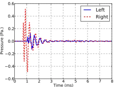
at 45◦ is shown in Figure 2.4.
The notion that localisation on the horizontal plane is dominated by ITD
0 1 2 3 4 5 6 7 8 Time (ms)
0.6 0.4 0.2 0.0 0.2 0.4 0.6
Pressure (Pa.)
[image:43.595.220.419.66.206.2]Left Right
Figure 2.4: Binaural Impulse Response (BIR) for a source positioned at 45◦ from a Kemar mannikin, obtained from the MIT HRTF catalogue (Gardner et al., 1994).
originally suggested by Rayleigh (1896). Whilst the roots of sound localisation
study appear long before Rayleigh, it is common to think of duplex theory as the
first scientifically verified theory of sound localisation. For an articulate historical
review see (Gulick, 1971; Hickson and Newton, 1981). When a sound source is
presented at a certain angle from the listener, there will be a difference in the
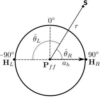
propagation paths between the source and each of the listener’s ears7, as shown in Figure 2.8. This results in inter-aural differences in time and level of arrival,
which provide the foremost cues for localisation on the horizontal plane.
Accord-ing to Duplex Theory, localisation at low frequencies is dominated by interaural time differences (ITDs) whereas localisation at high frequencies is dominated by
interaural level differences (ILDs) due to the shading effects of the head.
Whilst considered a landmark achievement, duplex theory cannot explain how
the auditory system resolves front-back confusion and localisation in the median
plane. This suggests that other cues are also involved. The role of the pinna
in sound localisation have been thoroughly studied in (Angell and Fite, 1901;
Batteau, 1967; Fisher and Freedman, 1968; Blauert, 1970) showing that the
ge-ometric structure of the pinna causes variance in the signal’s response. In other
words, the main function of the pinna in sound localisation is to modify the
spectral contents of the input signal according to the direction of arrival of the
incident wave, effectively resulting in an angle-dependent transfer function. This
Left Ear Right Ear Source
Figure 2.5: Illustration of the different propagation paths from a source to the two ears of a listener, resulting in interaural time and level differences.
is accomplished by superposition of a direct wave and a wave diffracted within
the unique structure of the pinna, which results in a different propagation path
for different angles of arrivals. The difference in path length between the direct
and diffracted components cause a phase difference, which manifests itself in a
different comb-filter structure for different incidence angles when the two compo-nents are summed together. Additional cues include head movements and visual
information (Wallach, 1940), however these are less related to this work.
Cue Encoding in the Brainstem
In physiological terms, interaural differences are reflected in differences between
signals transmitted through the ipsilateral and contralateral auditory nerves,
whereas monaural cues are encoded within the spectral contents of the signals
themselves. This leaves the central auditory system with an immense amount
of information to process, and not surprisingly, the neural pathway of spatial
processing is quite complicated. Since the perceptual models discussed in this
thesis are analytically-motivated, a rather simplified overview of the neural
pro-cesses corresponding to sound localisation would suffice. An illustration of the
ascending auditory pathway in the central nervous system is shown in Figure 2.6.
Auditory nerve fibres connect the cochlea to the first processing area in the
CN MGB
IC
SOC
CN MGB
IC
SOC
Cortex Cortex
Figure 2.6: Simplified illustration of the ascending auditory pathway. CN, cochlear nucleus; SOC, superior olivary complex; IC, inferior colliculus; MGB, medial geniculate body. Solid lines - ipsilateral pathway; Dotted lines - con-tralateral pathway. Figure based on (Schnupp et al., 2010)
each playing a different role in the analysis of the signal’s acoustic properties, such
as spectral content, signal onset, temporal structure and periodicity, to name a
few. Information from the CN is then projected to the superior olivary complex
(SOC) which plays an important role in the processing of binaural cues.
Encod-ing of ILDs occur at the lateral superior olive (LSO), whereas encoding of ITDs occur at themedial superior olive (MSO). The neural pathways for these cues are shown schematically in Figure 2.7. It is important to recall that information is
transmitted from the cochlea in separate frequency channels, meaning that
pro-cessing in these brainstem areas should also be carried out in different frequency
bands. In fact, throughout the auditory pathway, regions of the brain
process-ing different frequencies are topologically located along an axis representprocess-ing the
frequencies they process. This is referred to as a tonotopic arrangement.
Neurons of the LSO are excited by signals from the ipsilateral ear but are
inhibited by signals from the contralateral ear. Cells of theanteroventral cochlear nucleus (AVCN) provide excitation bilaterally, however the connection of con-tralateral AVCN to the LSO is relayed through themedial nucleus of the trapezoid body (MNTB) which make the projection inhibitory. This excitation-inhibition
(EI) process is the basis of encoding ILD cues in the LSO. For example, if the
AVCN
LSO
MNTB
AVCN MSO
Ipsilateral (excitatory) Contralateral (excitatory) Inhibitory
Figure 2.7: Schematic representation of ILD and ITD processing in the auditory brainstem. AVCN, anteroventral cochlear nucleus; MNTB, medial nucleus of the trapezoid body; LSO, lateral superior olive; MSO, medial superior olive. For visual clarity, pathway is shown only for the ipsilateral side. Figure based on (Yin, 2002).
there would be an equal amount of excitation and inhibition, resulting in a low
firing rate. As the source is moved towards the ipsilateral ear, the increase in
ILD will manifest itself in more excitation and less inhibition. Since excitation
and inhibition essentially affect a neuron’s firing rate, then ILDs are represented
as rate-coding in LSO neurons.
Encoding of ITD cues is somewhat more complicated, and the exact process
is still not entirely agreed upon. Perhaps the most widely accepted
explana-tion relies on a landmark model suggested by Jeffress (1948), whose underlying
assumption is that MSO neurons act as coincidence detectors. In contrast to
the LSO, the MSO receives excitatory inputs bilaterally, meaning that its
neu-rons fire at a maximal rate when ipsilateral and contralateral excitation occurs
at the same time. If one considers a single MSO neuron, then the transmission
path length from the ipsilateral and contralateral AVCNs depends on the
physi-cal location of the neuron. For example, a neuron who is equidistant from both
AVCNs will respond well when there is no interaural delay, and a neuron which is
physically closer to the ipsilateral side will respond well if the interaural delay is
biased against the contralateral side, essentially compensating for the difference
excitation-excitation (EE-type) neurons are thought to be tuned to specific ITD values, or best delays. This suggests that ITD is represented in the form of a
place code, in which different neural assemblies (residing in different places in the MSO) are activated as a response to different interaural delay times.
Higher Processing in the Midbrain and Cortex
The MSO and LSO effectively encode binaural cues and as such, provide more
refined directional information to upper stages of the auditory system. Still, in
order to localise a sound these data should be mapped to corresponding spatial
positions. The inferior colliculus (IC) is an area of convergence for different pathways, including outputs of the LSO and MSO, and is the first area where
binaural and monaural cues are integrated. There is physiological evidence drawn
from experiments in barn owls, that IC neurons are tuned to specific combinations
of ITDs and ILDs (Pe˜na and Konishi, 2002), effectively establishing a map of the
surrounding auditory space8. Furthermore, in the IC of such species, information delivered across different frequency channels is integrated.
This, however, is not the end of the auditory pathway involving sound
lo-calisation. Visual cues play an important role in sound localisation, as well as
feedback from head movements. The IC of mammals is linked to a multisensory
structure in the midbrain, called the superior colliculus (SC). This area features neural maps of the visual space, and controls reflexes such as eye and head
move-ments, which provide an improved means of auditioning localisation cues. It is
understandable that all of these processes occur subcortically, as reflex behaviour
is essential for survival. Yet, the auditory cortex (A1) also contributes to sound
localisation, in addition to being responsible for our ability to identify sounds.
Nevertheless, as higher stages of the analytical model presented in this thesis are
not explicitly related to neurophysiological evidence of processes occuring in the
cortex, a detailed review of auditory processing in the cortex is outside the scope
of this chapter.