International Journal of Mechanical and Materials Engineering (IJMME), Vol. 4 (2009), No. 3, 249-255
APPLICATION OF ARTIFICIAL NEURAL NETWORK TO PREDICT BRAKE SPECIFIC
FUEL CONSUMPTION OF RETROFITTED CNG ENGINE
M. I. Jahirul, R. Saidur and H. H. Masjuki
Department of Mechanical Engineering University of Malaya,
50603 Kuala Lumpur, Malaysia Email: [email protected]
ABSTRACT
In this paper the applicability of artificial neural networks (ANN) is investigated for a retrofitted compressed natural gas (CNG) fueled spark ignition (SI) internal combustion engine (ICE). A four cylinder carbureted petrol engine is converted to run with NG and used throughout the work. The neural networks toolbox of Matlab 6.5 is used to develop and test the ANN model on a personal computer. An optimal design is completed for the 3 to 12 hidden neurons on single hidden layer with six different algorithms: batch gradient descent (GD), resilient back-propagation (RP), levenberg-marquardt (LM), batch gradient descent with momentum (GDM), variable learning rate (GDX), scaled conjugate gradient (SCG) in the back-propagation neural network model. The training data for ANN is obtained from experimental measurements. Engine speed (rpm), throttle position, fuel-air equivalence ratio (φ) and torque (N-m) were used in input layer while break specific fuel consumption (gm/kWh) was used as output layer. Statistical analysis in terms of Root-Mean-Squared (RMS), absolute fraction of variance (R2), as well as mean percentage error is used
to investigate the prediction performance of ANN. LM algorithm with 10 neurons on single hidden layer in back-propagation of ANN model has shown best result in the present study. The degree of accuracy of the ANN model in prediction is proven acceptable in all statistical analysis and shown in results. So, it can be concluded that ANN provides a feasible method in predicting specific fuel consumption of CNG driven SI engine.
Keywords: Internal combustion engine (ICE),
Compressed natural gas (CNG), Artificial neural network (ANN) and Specific fuel consumption (SFC)
1. INTRODUCTION
It is well known that fossil fuel reserves all over the world are diminishing at an alarming rate and a shortage of crude oil is expected within the next few decades. The world total natural gas (NG) reserve as of January 1, 2007 was 6,183 Tscf and based on the current
consumption rates, the estimated total recoverable gas, including proven reserves is adequate for about 66.7 years (IEO,2008). This has resulted in an increased interest to use CNG as fuel for internal combustion engines. The merits of CNG as an automotive fuel over conventional fuels are many and presented comprehensively by Nylund et al. (2002) and Aslam et al.
(2003). Due to some of its favorable physio-chemical properties, CNG appears to be an excellent fuel for the spark ignition (SI) engine. Moreover, SI engines can be converted to CNG operation quite easily with the addition of a second fueling system. CNG has been used in vehicles since 1930’s and the current worldwide NGV population is more than 4.5 million according to the International Association for Natural Gas Vehicle (IANGV) statistics and this figure is fast increasing everyday ( Aslam et al., 2006).
To investigate experimentally the performance of an engine is complex, time consuming and costly, especially for studies, which use many, different blends. Therefore, a mathematical model is used to predict the performance and emissions of the engines. But, the resulting accuracies may not always be satisfactory. One alternative to the mathematical model is the experiment-based approach, such as artificial neural-networks (ANNs). Neural networks are nonlinear computer algorithms, which can model the behavior of complicated nonlinear processes. For the development of high speed digital computers, the application of ANN approach could be progressed at a very impressive rate. In recent years, this method has been applied to various disciplines including automotive engineering, in forecasting of engine thermal characteristics for different working conditions. Some researchers studied this method to predict internal combustion engine characteristics. Artificial neural network approach has been used by Yuanwang et al. (Aslam et Al., 2006), to analyze the
effect of cetane number on exhaust emissions from engine, Lucas et al. (Yuanwang et al., 2003), to model
Diesel particulate emission, Hafner et al. (Lucas et al.,
2001), for diesel engine control design, Shayler et. al.
throttle body processes in an automotive engine. Those studies do not need an explicit formulation of the physical relationships of concerned problems. Several studies have also used ANNs in different engineering areas (Sozen et. al., 2005).
[image:2.612.57.294.255.428.2]In the existing literatures, it was shown that the use of ANN is a powerful modeling tool that has the ability to identify complex relationships from input–output data. However, no investigation to predict engine specific fuel consumption (SFC, gm/kWh), retrofitted CNG fueled IC engine using ANN approach appears to have been published in the literature to date. Therefore, the present work investigates the applicability of ANN method for predicting the specific fuel consumption parameter.
Figure 1:Layout of the experimental setup
2. EXPERIMENTAL SETUP AND TEST
PROCEDURE
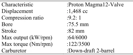
The layout of the experimental setup has shown in Figure 1. The test engine has been converted from a gasoline (Proton Magma) engine and has been equipped with a bi-fuelling system. The main specifications of the test engine are listed in Table 1.
Table 1: Specifications of the research engine
Characteristic Displacement Compression ratio Bore Stroke
Max output (kW/rpm) Max torque (Nm/rpm) Carburetor
:Proton Magma12-Valve :1,468 cc
:9.2: 1 :75.5 mm :82 mm :64/6000
:122/3500 :Down-draft 2-barrel
An AG 150 (Froude Consine) eddy-current dynamometer has been used for testing the engine. All the electronic equipment, together with its manipulative controls and
indicators, etc was mounted on ‘CP Cadet10’ control unit. The engine has been operated at constant throttle 30%, 40%, and 50% and 100% with a variable speed range of 1500-3500 RPM at a constant increment of 100 RPM. CNG consumption has been measured with Kobold gas flow meter (Model WFM 2705). The CNG flow meter was incorporated with engine control system through interface cards. A PC-based data acquisition and control system has been used for controlling all the operation regarding the test where every stage was allowed to run around 6–8 min with updating data in every 30 s. Torque, power and fuel consumption have been measured to calculate SFC.
3. ARTIFICIAL NEURAL NETWORKS
A widely used NN model called the multi-layer perception (MLP) NN is shown in Figure 2. The MLP type NN consists of one input layer, one or more hidden layer (s) (middle) in between input and output layers and one output layer. Each layer employs several neurons (nodes), and each neuron in a layer is connected to the neurons in the adjacent layer with different weights. The weights, after training, contain meaningful information, whereas before training they are random and have no meaning (Erol et al., 2004).
Signals flow into the input layer, pass through the hidden layer(s), and arrive at the output layer. With the exception of the input layer, each neuron receives signals from the neurons of the previous layer. The incoming signals or input (xij) are multiplied by the weights (vij)
and summed up with the bias (bj) contribution.
Mathematically it can be expressed as:
j ij
n
i
i
V
b
X
+
=
∑
=1
j
net
(1)The output of a neuron is determined by applying an activation function to the total input and calculated using Equation 1 (Kreider et al., 1992). If the computed outputs
do not match the known (i.e. target) values, NN model is
in error. Then, a portion of this error is propagated backward through the network. This error is used to adjust the weight and bias of each neuron throughout the network so the next iteration error will be less for the same units. The procedure is applied continuously and repetitively for each set of inputs until there are no measurable errors, or the total error is smaller than a specified value.
[image:2.612.54.287.587.683.2]network together with the desired output: the weights and bias values are initially chosen randomly and the weights adjusted so that the network produces the desired output. After training, the weights contain meaningful information, contrary to the initial stage where they are random and meaningless. When a satisfactory level of performance is reached, the training stops, and the network uses the weights to make decisions.
Figure 2: Architectural graph of a Multilayer Perception (MLP) with one hidden layer
4. APPLICATION OF NEURAL NETWORKS IN
THE PRESENT STUDY
Three data sets are needed for ANNs: for training, validation and testing the network. The usual approach is to prepare a single data-set, and differentiate it by a random selection. In this study, the experimental results mentioned above were used to train, validate and test an artificial neural-network. Engine speed (rpm), throttle position, fuel-air equivalence ratio and torque (N-m) are used in input layer while break specific fuel consumption (gm/kWh) used as output layer. The learning algorithm called the back-propagation was applied for the single hidden layer. Batch gradient descent (GD), resilient backpropegation (RP), levenberg-marquardt (LM), batch gradient descent with momentum (GDM), variable learning rate (GDX), scaled conjugate gradient (SCG) algorithms have been used for the variants. The Neural Network has been optimized using the MATLAB Version 6.5 Neural Network Toolbox. In the training stage, to define the output accurately, we tried to increase the number of neurons step-by-step (i.e 3–12) in the hidden layer. Inputs and outputs have been normalized in the range of (0.1–0.9) as NN works efficiently within this
[image:3.612.303.569.199.730.2]range. Neurons in the input layer have no transfer function. Logistic sigmoid (logsig) transfer function has been used in hidden layer while purelinear (purelin) transfer function has been used in output layer. After the successful training of the network, the network was tested with the test data. Using the results produced by the network, statistical methods have been used to make comparisons.
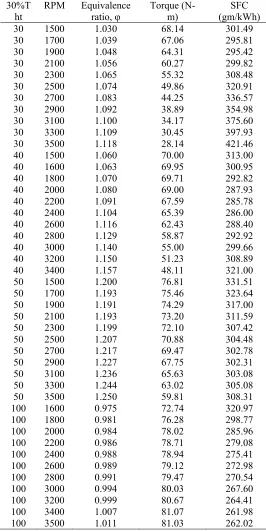
Table 2: Data sets used for training the network
30%T
ht RPM Equivalence ratio, φ Torque (N-m) (gm/kWh) SFC
30 1500 1.030 68.14 301.49
30 1700 1.039 67.06 295.81
30 1900 1.048 64.31 295.42
30 2100 1.056 60.27 299.82
30 2300 1.065 55.32 308.48
30 2500 1.074 49.86 320.91
30 2700 1.083 44.25 336.57
30 2900 1.092 38.89 354.98
30 3100 1.100 34.17 375.60
30 3300 1.109 30.45 397.93
30 3500 1.118 28.14 421.46
40 1500 1.060 70.00 313.00
40 1600 1.063 69.95 300.95
40 1800 1.070 69.71 292.82
40 2000 1.080 69.00 287.93
40 2200 1.091 67.59 285.78
40 2400 1.104 65.39 286.00
40 2600 1.116 62.43 288.40
40 2800 1.129 58.87 292.92
40 3000 1.140 55.00 299.66
40 3200 1.150 51.23 308.89
40 3400 1.157 48.11 321.00
50 1500 1.200 76.81 331.51
50 1700 1.193 75.46 323.64
50 1900 1.191 74.29 317.00
50 2100 1.193 73.20 311.59
50 2300 1.199 72.10 307.42
50 2500 1.207 70.88 304.48
50 2700 1.217 69.47 302.78
50 2900 1.227 67.75 302.31
50 3100 1.236 65.63 303.08
50 3300 1.244 63.02 305.08
50 3500 1.250 59.81 308.31
100 1600 0.975 72.74 320.97
100 1800 0.981 76.28 298.77
100 2000 0.984 78.02 285.96
100 2200 0.986 78.71 279.08
100 2400 0.988 78.94 275.41
100 2600 0.989 79.12 272.98
100 2800 0.991 79.47 270.54
100 3000 0.994 80.03 267.60
100 3200 0.999 80.67 264.41
100 3400 1.007 81.07 261.98
Table 3: Data sets used for validation
30%Tht 30%Tht
RPM Equivalence ratio, φ Torque (N-m) (gm/kWh) SFC
30 1600 1.034 67.84 297.95
30 2000 1.052 62.43 297.05
30 2400 1.070 52.63 314.26
30 2800 1.087 41.52 345.46
30 3200 1.105 32.16 386.58
40 1900 1.075 69.43 306.44
40 2300 1.097 66.59 290.00
40 2700 1.123 60.71 285.61
40 3100 1.145 53.07 290.39
40 3500 1.160 47.00 303.94
50 1800 1.191 74.86 327.42
50 2200 1.196 72.66 314.14
50 2600 1.212 70.21 305.80
50 3000 1.232 66.74 302.39
50 3400 1.247 61.50 303.93
100 1700 0.978 74.79 308.45
100 2100 0.986 78.45 281.97
100 2500 0.989 79.02 274.14
100 2900 0.993 79.73 269.13
100 3300 1.003 80.92 263.01
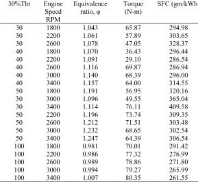
Table 4: Data sets use for test network
30%Tht Engine Speed
RPM
Equivalence
ratio, φ Torque (N-m) SFC (gm/kWh)
30 1800 1.043 65.87 294.98 30 2200 1.061 57.89 303.65 30 2600 1.078 47.05 328.37 40 1800 1.070 36.43 296.44 40 2200 1.091 29.10 286.54 40 2600 1.116 69.87 286.94 40 3000 1.140 68.39 296.00 40 3400 1.157 64.00 314.55 50 1800 1.191 56.95 320.16 30 3000 1.096 49.55 365.04 30 3400 1.114 76.11 409.58 50 2200 1.196 73.74 309.35 50 2600 1.212 71.51 303.48 50 3000 1.232 68.65 302.54 50 3400 1.247 64.39 306.54 100 1800 0.981 70.01 291.42 100 2200 0.986 77.32 276.99 100 2600 0.989 78.86 271.80 100 3000 0.994 79.27 265.99 100 3400 1.007 80.35 261.55
5. MEASURES OF PREDICTION
PERFORMANCE
Using the results produced by the network, statistical methods have been used to investigate the prediction
performance of NN results. To judge the prediction performance of a network, several performance measures are used. Those include statistical analysis in terms of Root-Mean-Squared (RMS), absolute fraction of variance (R2), as well as mean error percentage values [11]. Those
are defined bellow:
(
)
⎟⎟⎟ ⎟ ⎟ ⎠ ⎞ ⎜⎜ ⎜ ⎜ ⎜ ⎝ ⎛ − − − =∑
∑
= = = = 2 1 2 1 2 ) ( 1 N I I M a p a N i i E E E ER (3)
(
)
N
E
E
RMS
N i i p a∑
= =−
=
1 2 (4)∑
= =⎟
⎟
⎠
⎞
⎜
⎜
⎝
⎛
×
−
=
i Ni a p a
E
E
E
1100
N
1
Error
%
Mean
(5)where
Ea-Actual result Ep-Predicted result Em-Mean value N-Number of pattern
The coefficient of multiple determinations R2 compares
the accuracy of the model to the accuracy of a trivial benchmark model. A perfect fit would result in an R2
value of 1 and a very good fit near 1.
6. RESULTS AND DISCUSSIONS
[image:4.612.24.313.390.655.2]conjugate gradient (SCG) algorithms. The testing accuracy of trained networks is shown in Figs. 4-6.
[image:5.612.333.572.266.446.2]Figure 3: Network training cycles
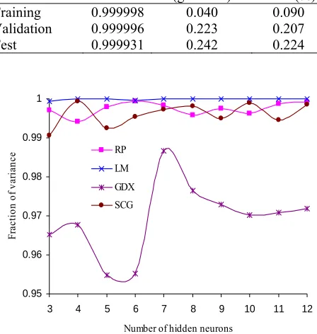
Table 4: Performance of optimized network
R2 RMS
(gm/kWh) Error (%) Mean
Training 0.999998 0.040 0.090
Validation 0.999996 0.223 0.207
Test 0.999931 0.242 0.224
0.95 0.96 0.97 0.98 0.99 1
3 4 5 6 7 8 9 10 11 12
Number of hidden neurons
Fr
ac
ti
on of
va
ri
anc
e RP
[image:5.612.49.291.368.427.2]LM GDX SCG
Figure 4: R2 value of test for different algorithms with
increasing number of hidden layer.
The performances of GD and GDM were not in satisfactory level and the statistical values were out of the range for Figs. 5-6. The accuracies of algorithms RP, GDX and SCG have shown good result but not consistent with hidden neurons. LM algorithm has shown good
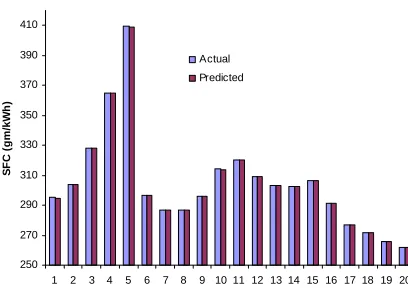
performance accuracy and consistency with changing number of hidden neurons. The best network was found to be the LM algorithm with 10 hidden neurons. In Table 4, the statistical values of the outputs for this algorithm have been shown for the training, validation and testing data. The actual and predicted outputs of training and testing have been shown graphically in Figs. 7-8. The ANN predictions for the BSFC yield a mean relative error of 0.224%, a root mean square error of 0.242 gm/kWh and a correlation coefficient of 0.999931. These values show that the ANN predicts the BSFC quite well despite wide ranges of operating conditions. It is clear that the performance of the ANN would have been even better, if a higher number of test runs had been performed to provide a larger amount of experimental data for the network training.
0 5 10 15 20 25 30
3 4 5 6 7 8 9 10 11 12
Number of hidden neurons
RM
S
RP LM
GDX SCG
Figure 5: RMS value of test for different algorithms with
increasing number of hidden layer.
0 0.2 0.4 0.6 0.8 1 1.2
3 4 5 6 7 8 9 10 11 12
Number of hidden neurons
M
ean
p
er
cen
tag
e er
ro
r (
%
)
RP
LM
GDX
SCG
[image:5.612.63.287.390.626.2] [image:5.612.336.559.498.678.2]250 270 290 310 330 350 370 390 410 430 450
1 3 5 7 9 11 13 15 17 19 21 23 25 27 29 31 33 35 37 39 41 43
SF C (g m /k Wh ) Actual Predicted
Figure 7: Comparison of actual and predicted values for BSFC of training data
250 270 290 310 330 350 370 390 410
1 2 3 4 5 6 7 8 9 10 11 12 13 14 15 16 17 18 19 20
[image:6.612.66.278.75.251.2]SF C ( g m /k W h ) Actual Predicted
Figure 8:Comparison of actual and predicted values for BSFC test data.
The formulations of the outputs obtained from the weights are given using Eqs. 5–6.
0.7597) -8742 . 1 3647 . 0 8952 . 0 5182 . 0 1241 . 0 2199 . 0 4424 . 1 3337 . 2 1048 . 0 3928 . 2
( 1 2 3 4 5 6 7 8 9 10
1 1 F F F F F F F F F F e BSFC + + − − + − − + − − − + = (6)
Where Fi = ( i = 1,2,3…….10) can be calculated according to
equation (7). i E i
e
F
−+
=
1
1
(7)Where Ei is the weighted sum of the of the input and is given by
[image:6.612.67.271.321.465.2]equation as seen in the Tables 5.
Table 5. The weights (C) between input layer and hidden layer for BSFC
Ei = C1Tht + C2Ns + C3φ + C4T + C5
i
C1 C2 C3 C4 C5
1 -2.8529 7.5086 -21.2481 -4.057 8.8613 2 2.7587 -4.0614 0.9233 10.9504 -5.2455 3 -10.0031 -1.9646 -26.0019 6.8492 5.1912 4 2.6867 8.1041 -32.6024 -2.9196 8.9578 5 -4.6516 5.9319 -14.4598 8.387 -0.2843 6 3.8218 -7.2814 7.8886 -13.59 6.5203 7 -5.2524 -7.9815 28.3589 4.1564 0.4495 8 6.7635 -4.7433 28.1554 1.8058 -8.1378 9 -4.5086 8.1115 19.0278 2.344 -8.1517 10 4.3511 -7.246 -26.3438 -5.1709 11.8424
7. CONCLUSION
The aim of this paper has been to show the possibility of using the neural networks for predictions of dual fuel engine performance. The network produces the predicted results of brake specific fuel consumption parallel to the experimental ones. The RMS error values are smaller
than 0.05 gm/kWh, R2 values are about 0.9999 and mean
error smaller than 0.25%, which may easily be considered within the acceptable range. A back propagation (BP) neural network model with GD, RP, LM, GDM, GDX and SCG algorithms have been studied in single hidden layer. Number of neurons on hidden layer also varied to optimize network. In most cases, the best results were obtained from the LM algorithm. On the other hand GD and GDM algorithoms showed very poor prediction performance. The overall results show that the networks can be used as an alternative for predicting the performances of CNG fueled internal combustion engine.
The result of this study shows that ANN has ability to learn and generalize a wide range of experimental conditions. Therefore, the usage of ANNs may be highly recommended to predict the engine performance instead of having to undertake complex and time-consuming experimental studies.
ACKNOWLEDGEMENT
REFERENCE
Aslam M.U, Masjuki H.H, Kalam M.A, Abdesselam H., Mahlia T.M.I, Amalina M.A., 2006. An experimental investigation of CNG as an alternative fuel for a retrofitted gasoline vehicle. Fuel, . vol 85, pp.717–724.
Aslam MU, Masjuki HH, Maleque MA, Kalam MA, Mahlia TMI, Zainon Z, 2003. Introduction of natural gas fueled automotive in Malaysia. Proc. TECHPOS’03. 160, UM, Malaysia.
Erol Arcakhoglu, Abdullah Cavusoglu, Ali Erisen. 2004 Thermodynamic analyses of refrigerant mixtures using artificial neural-networks. Applied Energy. vol. 78, pp.
219–30.
International Energy Outlook, 2008. International Energy Outlook Energy information administration. Washington, DC: Department of Energy; www.eia.doe.gov , Dater 15/08/2008
Kreider JF, Wang XA. 1992. Artificial neural networks demonstrations for automated generation of energy use predictors for commercial buildings. ASHRAE
Transactions. . vol. 97(1), pp. 775–9.
Lucas A., Duran M., Carmona, M. Lapuerta M, 2001. Modeling diesel particulate emissions with neural networks, Fuel, vol. 4: pp. 548–593.
Nylund N.O., Laurikko J., Ikonen M., 2002. Pathways for natural gas into advanced vehicles. IANGV
(International Association for Natural Gas Vehicle) Edited Draft Report
Shayler P. J, Goodman M., Ma T., 2000 The exploitation of neural networks in automotive engine management systems, Eng. Appl. Artif. Intell. vol. 13, pp 147–151.
Sozen A, Arcakhoglu E., 2005. Prediction of solar potential in Turkey. Appl Energ, 2005. vol. 80, pp. 35–45.
Tan Y., Saif M., 2000. Neural-networks-based nonlinear dynamic modeling for automotive engines,
Neurocomputing. vol. 30, pp.129–142.
Yuanwang D., Meilin Z., Dong X., Xiaobei C., 2003. An analysis for effect of cetane number on exhaust emissions from engine with the neural network, Fuel. vol 81, pp.
1963–1970.