Identification of Growth Rate of Plant based on leaf features using Digital Image Processing Techniques

(1)

International Journal of Emerging Technology and Advanced Engineering

Website: www.ijetae.com (ISSN 2250-2459,ISO 9001:2008 Certified Journal, Volume 3, Issue 8, August 2013)

266

Identification of Growth Rate of Plant based on leaf

features using Digital Image Processing Techniques

Ms Smita Patil

1

, Prof. Shridevi Soma

2

, Prof. Suvarna Nandyal

3 1

Student VTU RO, Gulbarga

2,3_{PDA College of Engg, Glb}

Abstract - Plant recognition and determining their growth rate is a challenging research work, which helps farmers to take important decisions such as pesticide spray, fertility, manure spraying etc. in the agriculture. Normally growth rate of plant is identified by measuring the height of the plant with regular intervals, but in this work it is proposed that growth rate can also be predicted based on leaf size and color. Hence the leaf features are used for the same task. Color and Texture features were incorporated for the identification of the leaf. A digital camera is used to acquire the leaf images. The proposed approach consists of four phases such as preprocessing, segmentation, feature extraction and classification. The preprocessing phase involves image transformation and resize. In order to extract leaf shape and boundary features, leaf has to be segmented from a plant. Hence the watershed algorithm is used for segmentation. For feature extraction phase the color and texture features are derived. Total of 141 features are extracted in which 121 color features are taken using histogram and 20 texture features using Discrete Wavelet Transform and Fast Fourier Transform and are given as input vector to the Support Vector Machine classifier. The ultimate goal of this work is to develop a system where a user in the field can take a picture of a plant leaf, feed it to the machine vision system carried on a portable computer, and have the system to classify and identify the growth rate. The classification accuracy of 94.73% is observed.

Keywords - Color features, Image Preprocessing, Leaf Classification, SVM, Segmentation, Texture features.

The paper is organised into seven sections. Section 1 gives Introduction and Literature Survey, Section 2 presents Leaf capturing, Section 3 tells about proposed design, Section 4 describes about Image pre-processing and Segmentation, Section 5 deals with Feature Extraction, Section 6 describes about results and discussion and Conclusion is presented in Section 7.

I. INTRODUCTION

Plants play a vital role in the environment. There will be no existence of the earth‟s ecology without plants. However, recently, several species of plants are at the danger of extinction. In order to protect plants and to catalogue various species of flora diversities, a plant database becomes very essential. There is huge volume of plant species worldwide.

In order to handle such volumes of information, development of a rapid and competent classification technique has become an active area of research. Moreover, along with the conservation feature, recognition of plants has also become essential to exploit their medicinal properties and using them as sources of alternative energy sources like bio-fuel. There are various ways to recognize a plant, like flower, root, leaf, fruit etc. Recently, computer vision and pattern recognition techniques have been applied towards automated process of plant recognition [2].

Shape, color and texture features are common features involved in several applications. However, some researchers used part of those features only. Invariant moments are very popular in image processing to recognize objects, including leaves of plants. Color was included in several applications as features, for which image correlogram was used for image retrieval, and color moments were used for plant classification [1].

The classification of plant leaves is a vital mechanism in botany and in tea, cotton and other industries. Additionally, the morphological features of leaves are employed for plant classification or in the early diagnosis of certain plant diseases. Leaf recognition plays an important role in plant classification and its key issue lies in whether the chosen features are constant and have good capability to discriminate various kinds of leaves. The recognition procedure is very time consuming. Computer aided plant recognition is still very challenging task in computer vision because of improper models and inefficient representation approaches.

II. LITERATURE SURVEY

(2)

International Journal of Emerging Technology and Advanced Engineering

267

A leaf classification system using shape, vein , color and texture features was developed by Abdul Kadir et al., [3]. A prominent result was obtained using Probabilistic Neural Network. Stephen Gang Wu et al., [4] proposed work on leaf recognition using PNN. 12 leaf features are extracted and orthogonalized into 5 principal variables which consist the input vector of the PNN. The PNN is trained by 1800 leaves to classify 32 kinds of plants with accuracy greater than 90%.

Arun Priya et al., [5] the proposed approach consists of three phases such as preprocessing: transforming to gray scale and boundary enhancement, feature extraction: derives the common DMF from five fundamental features and classification: Support Vector Machine (SVM) classification for efficient leaf recognition. 12 leaf features which are extracted and orthogonalized into 5 principal variables are given as input vector to the SVM.

From the literature survey we found, till now many work has been done on the identification and classification of plants.

III. CAPTURING LEAF IMAGE

The leaves samples are collected from the field using Digital camera of 14.1 MB pixels. The sample images are shown in the figure 1.

Rosa rubiginosa

Azadirachta indica

Prunus amygdalus

Mangifera indica

Polyalthia longifolia

Pelta phorum pterocarpum

Pongamia pinnata

Rosa sinensis

Figure 1: Sample Leaves

We have collected 80 images of 10 different classes containing leaf images in bundles. These images were captured in 4 different stages which gives variation in color and leaf size. An active contour segmentation is applied to segment a single leaf from the bundle. For training total of 4 stage * 10 types = 40 images are considered and all the 40 leaf images in bundle are given for testing.

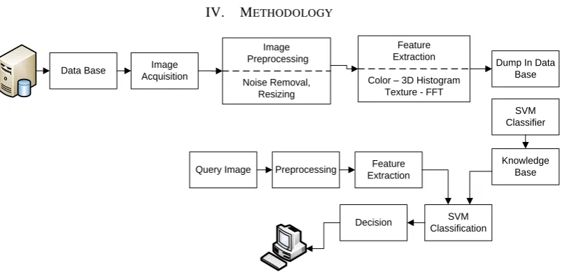
IV. METHODOLOGY

Data Base Image Acquisition

Dump In Data Base

SVM Classifier

Knowledge Base Query Image Preprocessing Feature

Extraction

SVM Classification Decision

Image Preprocessing

Noise Removal, Resizing

Feature Extraction

[image:2.595.98.500.472.670.2]

Color – 3D Histogram Texture - FFT

Figure 2: Proposed Design

From the figure 2 it is evident that Support Vector Machine is the core for this system.

(3)

International Journal of Emerging Technology and Advanced Engineering

268

V. PRE-PROCESSING AND SEGMENTATION

The leaf image pre-processing refers to the initial processing of input leaf image to correct the geometric distortions, calibrate the data radio metrically and eliminate the noise and clouds that present in the data, these operations are called pre-processing because they are normally carried out before the real analysis and manipulations of the image data that is considered to extract any specific information. The aim is to correct the distorted or degraded image data to create a more faithful representation of the real leaf which increase classification accuracy.

Several techniques like boundary enhancement, smoothening, filtering, noise removal, etc exists, but in our work we have used Pre-processing techniques like Resizing and Color conversion.

A.Resizing

The most obvious and common way to change the size of an image is to resize or scale an image. The content of the image is then enlarged or more commonly shrunk to fit the desired size. But while the actual image pixels and colors are modified, the content represented by the image is essentially left unchanged.

However resizing images can be a tricky matter. It can modify images in very detremental ways, and there is no 'best way' as what is best is subjective as to what you actually want out of the resize process.

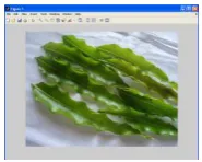
In this work Bilinear Interpolation method is used for resizing the image by 200 X 200 image pixel. Figure-4 is the resultant of Resize Operation.

[image:3.595.51.144.510.584.2]

Figure 3: Image before resize Figure 4: Image after resize

For convenience take all the leaf images to be of the same size and resolution. Plants are basically classified according to shapes, colors and structures of their leaves and flowers. In addition, the colors of leaves are always green shades and the variety of changes in atmosphere because the color features having low reliability. Therefore, to recognize various plants using their leaves, the obtained leaf image in RGB format will be converted to gray scale before pre-processing. The formula used for converting the RGB pixel value to its gray scale.

(1)

Where R, G, B corresponds to color components of the pixel respectively.

B.Color Conversion

Color:One of the most important features that make possible the recognition of images by humans is color. Color is a property that depends on the reflection of light to the eye and the processing of that information in the brain.

A color model is an abstract mathematical model describing the way colors can be represented as tuples of numbers, typically as three or four values or color components (e.g. RGB and CMYK are color models). However, a color model with no associated mapping function to an absolute color space is a more or less arbitrary color system with no connection to any globally understood system of color interpretation.

The different color spaces are used such as RGB and HSV. In this work we have used HSV color space for color features. HSV stands for Hue, Saturation, Value, it is a cylindrical-coordinate representation and is known for its intuitively i.e. close to how a person would describe a color.

HSV color space is a popular choice for manipulating color. The color space, representing hue, saturation and color value (brightness) has the shape of a hexagonal cone. This color space is used for a part of the color statistics given below:

Illuminant: value indicates the color of the light source. It is calculated in two versions, through the “Gray-world algorithm” and the “White patch algorithm”. The former is calculated by the mean of the three color channels, which is assumed to be “gray” (multiplied by 2 to get white), the latter is calculated by assuming that a white patch is always visible in an image, therefore taking the maximum value of each Channel.

Unique colors: this value is calculated by

transformation into the HSV-space and counting the unique values in the Hue channel.

Histogram sparseness: a histogram is calculated and bins containing counts higher than a fixed cut-off value counted.

Pixel saturation: this is calculated as a ratio between the number of highly saturated and unsaturated pixels in the HSV color space.

(4)

International Journal of Emerging Technology and Advanced Engineering

269

The brightness is determined by the colors vertical position in the cone. At the pointy end of the cone, there is no brightness, so all colors are black. At the fat end of the cone are the brightest colors.

Color Equations used in our work are as follows:

RGB to HSV conversion formula

The R, G, B values are divided by 255 to change the range from 0...255 to 0...1:

R' = R/255 G' = G/255 B' = B/255

Cmax= max(R', G', B')

Cmin= min(R', G', B')

Δ = Cmax - Cmin

Hue, Saturation and value calculation:

Watershed Segmentation Algorithm

The watershed algorithm can be directly

implemented by making use of morphological geodesic operators on successive thresholds of an image. A more efficient algorithm that uses queues of pixels to access those pixels which must be modified at each step is used in most practical implementations.

The image to which the watershed is applied should have each region of the partition to be computed marked by a greyscale minimum, and the boundaries of the regions marked by gray-scale maxima. As the image to be segmented usually does not satisfy these requirements, it is pre-processed to produce an image that better satisfies them.

To implement this transform, the classical algorithm “by swamping” proposed by Vincent has been used. The relief corresponding to the gradient modulus is progressively flooded with water springing from all local minima. During this flooding step, each time two flooded regions coming from different springs tend to merge, a virtual infinitely tall dam is raised up to keep them separate. At the end of the flooding, when each pixel has been reached by the water, the dam‟s network constitutes the watershed lines of the image segmentation.

Before the watershed transform. Basically, the idea is to reduce the number of seeds in the flooding algorithm in order to reduce the number of regions in the final segmentation. This is the markers approach.

In the proposed system an active contour watershed algorithm is applied at both testing and training phases iteratively to segment the region of interest.

VI. FEATURE EXTRACTION

The color and texture feature used in this work are presented in this work.

A.Color Feature

The color features are extracted using color histogram. Given a grayscale image, its histogram consists of the histogram of its grey levels; that is, a graph indicating the number of times each grey level occurs in the image. We can infer a great deal about the appearance of an image from its histogram. For pattern recognition applications, an HSV color histogram can be generated using an approach similar to the RGB color space. They utilize binary color sets to represent the color content as a color histogram. The H and S dimensions are divided into N and M bins, respectively, for a total of N×M bins. Each bin contains the percentage of pixels in the image that have corresponding H and S colors for that bin. Intersection similarity is used as a measure to capture the amount of overlap between two histograms.

In this work an RGB image is taken for the analysis, the RGB image is converted to HSV color space. The choice of taking the HSV image is attractive in theory. It is considered more suitable since it separates the color components (HS) from the luminance component (V) and is less sensitive to illumination changes, so extracting only H and S planes which represents color component of an image.

The hue scale is divided into eleven bins; saturation scale is divided into eleven bins. By combining each of these bins, a total of 121 features are used to represent a HSV color histogram.

These 121 features of all the training images are used for classification.

B.Texture Feature

The texture features are extracted using Discrete wavelet Transform and Fast Fourier Transform.

The DWT is a spatial-frequency decomposition that provides a flexible Multiresolution analysis of an image. In one dimension (1-D) the basic idea of the DWT is to represent the signal as a superposition of wavelets.

In a 2-D DWT, a 1-D DWT is first performed on the rows and then columns of the data by separately filtering and downsampling. This results in one set of approximation coefficients Ia and three sets of detail

coefficients. Ia, Ib and Ic represent the horizontal, vertical

(5)

International Journal of Emerging Technology and Advanced Engineering

270

In the language of filter theory, these four subimages correspond to the outputs of low-low (LL), low-high (LH), high-low (HL), and high–high (HH) bands. By recursively applying the same scheme to the LL sub band a multiresolution decomposition with a desires level can then be achieved. Therefore, a DWT with decomposition K levels will have M = 3*K+1 such frequency bands. The 2-D structures of the wavelet transform with two decomposition levels. It should be noted that for a transform with K levels of decomposition, there is always only one low-frequency band the rest of bands are high-frequency bands in a given decomposition level [6]. Once DWT is applied on the image we take LL band where we can get approximate coefficients of the image.

A Fast Fourier transform (FFT) is an algorithm to compute the discrete Fourier transform (DFT) and it‟s inverse. A Fourier Transform converts time (or space) to frequency and vice-versa; an FFT rapidly computes such transformations. As a result, Fast Fourier transforms are widely used for many applications in engineering, science, and mathematics. The FFT is an algorithm for calculating the complex DFT. The real DFT transforms an N point time domain signal into two point frequency domain signals. The time domain N/2+1 signal is called the time domain signal. The two signals in the frequency domain are called the real part and the imaginary part, holding the amplitudes of the cosine waves and sine waves, respectively. The FFT is based on the complex DFT, a sophisticated version of the real DFT. These transforms are named for the way each represents data that is, using complex numbers or using real numbers [17].

To obtain both real and imaginary part of the signal FFT is applied on the given image. The high energy will be at the corner of the image and it proceeds with that pixel and continue in the zigzag fashion to obtain the approximate image, form this approximate image 20 higher energy signals are considered as texture features.

First 20 higher energy signals are considered as texture features, 121 color features and 20 texture features, so total of 141 features are given to SVM classifier.

C.Classification

There are many classification techniques. In this work SVM is used for classification. SVMs have often been found to provide better classification results than other widely used pattern recognition methods, such as the maximum likelihood and neural network classifiers [4].

The main concepts of SVM are to first transform input data into a higher dimensional space by means of a kernel function and then construct an OSH (Optimal Separating Hyper Plane) between the two classes in the transformed space.

For plant leaf classification it will transform feature vector extracted from leaf‟s contour and texture. SVM finds the OSH by maximizing the margin between the classes.

The SVM approach seeks to find the optimal separating hyper plane between classes by focusing on the training cases that are placed at the edge of the class descriptors.

These training cases are called support vectors. Training cases other than support vectors are discarded. Let us consider a supervised binary classification problem. If the training data are represented by {xi, yi} i =

1, 2… N and yi € {-1, +1}.

Where N is the number of training samples, yi= +1 for

class w1 and yi= -1 for class W2. Suppose the two classes

are linearly separable. This means that it is possible to find at least one hyper plane defined by a vector W with a bias w0, which can separate the classes without error:

f(x) = w.x + w0 = 0 (2)

To find such a hyper plane, w and w0 should be

estimated in a way that yi(w.xi + w0) ≥ +1 for, yi = +1

(class w1) and yi(w.xi + w0) ≤ -1 for, yi = -1 ( class w2).

These two, can be combined to provide equation 3

yi (w.xi + w0) -1 ≥ 0 (3)

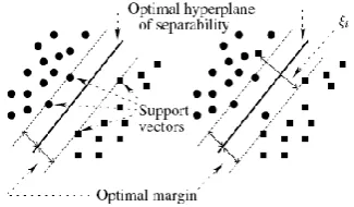
[image:5.595.349.512.489.584.2]

Many hyper planes could be fitted to separate the two classes but there is only one optimal hyper plane that is expected to generalize better than other hyper planes.

Figure 5: The case of linear separable classes.

The Support Vector Machine maps the input vector x into a high-dimensional feature space and then constructs the optimal separating hyper plane in that space. One would consider that mapping into a high dimensional feature space would add extra complexity to the problem. But, according to the Mercer‟s theorem, the inner product of the vectors in the mapping space can be expressed as a function of the inner products of the corresponding vectors in the original space.

The inner product operation has an equivalent representation: and is given as

Ǿ

(x)

Ǿ

(z)=

K(x, z)

(4)

(6)

International Journal of Emerging Technology and Advanced Engineering

271

Where K(x, z) is called a kernel function. If a kernel function K can be found, this function can be used for training without knowing the explicit form of Ǿ. We used RBF Kernel in SVM for Multiclass using OAA.

Multiclass SVM can be solved by combining the binary classification decision functions. Multiclass SVM is of two types namely, One againstOne decomposition and One against All decomposition. We are using one against all decomposition method for classification [2].

The OAA decomposition transforms the multiclass problem into a series of „c‟ binary subtasks that can be trained by the binary SVM. The OAA decomposition transforms the multiclass problem into a series of „c‟

Binary subtasks that can be trained by the binary SVM. Let l given the training set TyXY = {(x1,

y1‟)……… (xl,yl ‟

)} where xi € R n

and yi €

{1,……..,k}

is the class of xi, the i th

SVM solves the following problem:

Yi=











else

i

y

if

1 )

(

1

(5)

Where each binary data are trained by the SVM solver from the set TyXY , y € Y.

In this method, the One-Against-All reduction which creates one binary problem for each of the plant leaf classes. Then classifier for class i is trained to predict “Is the label i or not?” thus distinguishing examples in class i from all other examples.

VII. RESULTS AND DISCUSSIONS

In the quest for finding the best classification procedures and features for produce categorization, analyzes several features, color-, texture-, and shape-based image descriptors as well as diverse machine learning techniques such as Support Vector Machine (SVM) which is also utilized for the analysis of the classification.

Based on the dataset, 40 leaves are used for training. In this case, SVM is used as classifier. The dataset used in this approach is flavia and real dataset. Number of incorrect recognition is listed in the table.

The leaves are captured are in 4 different stages. The color Histogram and Discrete Wavelet Transform, Fast Fourier Transform used to extract color and texture features. Total of 141 features are used in this work.

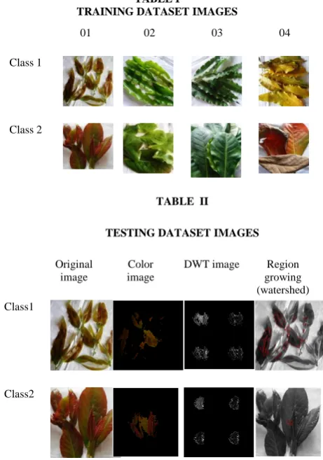
[image:6.595.319.550.263.592.2]

Table 1 and 2 give the sample training and testing images from Class 1 and 2. We can observe that application of Discrete Wavelet Transform and Watershed algorithm for segmentation during the test phase.

TABLE I

TRAINING DATASET IMAGES

01 02 03 04

Class 1

Class 2

TABLE II

TESTING DATASET IMAGES

Original image

Color image

DWT image Region growing (watershed) Class1

Class2

(7)

International Journal of Emerging Technology and Advanced Engineering

272

TABLE III

DETAILS ABOUT THE LEAF CLASSES AT DIFFERENT STAGES WITH THEIR ACCURACY

STAGE 1

Leaf name

Trainin g images

Testin g image

s

Incorrectl y classified

% of accurac

y

04 04 00 100

Prunus amygdalus

04 04 00 100

Pelta phorum pterocarpum

04 04 00 100

Mangifera indica

04 03 00 100

Pongamia pinnata

04 04 00 100

Cassia simea 04 04 00 100

Rosa rubiginosa

04 04 00 100

Azadirachta indica

04 04 00 100

Rosa sinensis 04 03 00 100

Psidum guava 04 04 00 100

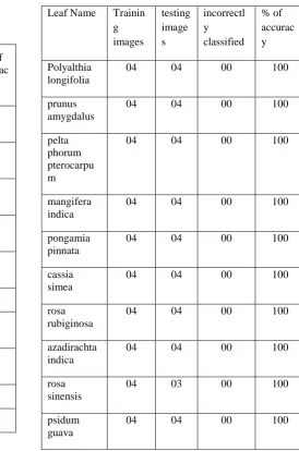
STAGE 2

Leaf Name Trainin

g images

testing image s

incorrectl y classified

% of accurac y

04 04 00 100

prunus amygdalus

04 04 00 100

pelta phorum pterocarpu m

04 04 00 100

mangifera indica

04 04 00 100

pongamia pinnata

04 04 00 100

cassia simea

04 04 00 100

rosa rubiginosa

04 04 00 100

azadirachta indica

04 04 00 100

rosa sinensis

04 03 00 100

psidum guava

[image:7.595.272.547.160.575.2]

(8)

International Journal of Emerging Technology and Advanced Engineering

273

STAGE 3

Leaf Name Trainin

g images

testing image s

incorrectl y classified

% of accurac y

04 04 00 100

prunus amygdalus

04 04 00 100

pelta phorum pterocarpu m

04 04 01 75

mangifera indica

04 03 00 100

pongamia pinnata

04 04 00 100

cassia simea

04 04 00 100

rosa rubiginosa

04 04 00 100

azadirachta indica

04 04 00 100

rosa sinensis

04 03 00 100

psidum guava

04 04 00 100

STAGE 4

Leaf Name Training

images

testing images

incorrectly classified

% of accuracy

04 04 00 100

prunus amygdalus

04 04 00 100

pelta phorum pterocarpum

04 04 00 100

mangifera indica

03 03 00 100

pongamia pinnata

04 04 00 100

cassia simea 04 04 00 100

rosa rubiginosa

04 04 01 75

azadirachta indica

04 04 00 100

rosa sinensis

03 03 00 100

psidum guava

(9)

International Journal of Emerging Technology and Advanced Engineering

274

From graph 1 to 4 we can observe the prominent results as for as the identification of the 10 leaf classes at four different stages.

PERFORMANCE GRAPH FOR STAGE 1

VIII. CONCLUSION

A method for identification of growth rate of leaf has been developed, which incorporates color, and texture features and uses SVM as a classifier. Histogram is used to extract color features and Discrete Wavelet Transform and Fast Fourier Transform for texture features extraction. The proposed work automatically classifies 10 kinds of leaves and their four stages for further analysis. The result gives 94.73% of accuracy which is much better than existing system. The proposed algorithm produces better accuracy and simple for execution. Although performance of the system is good enough and believe that the performance can still be improved. Further enhancement can be made by incorporating efficient features and kernel functions.

REFERENCES

[1] Abdul Kadir, Lukito Edi Nugroho, Adhi Susanto and Paulus Insap Santosa “Leaf Classification Using Shape, Color, and Texture Features” July to Aug Issue 2011.

[2] Arunpriya C and Antony Selvadoss Thanamani “An Efficient Leaf Recognition Algorithm for Plant Classification using support vector Machine” vol 2 Issue 2 feburary 2013.

[3] Iris R. Wang, Justin W. L. Wan and Gladimir V. G. Baranoski “Physically-based simulation of plant leaf growth” in the year 2004.

[4] Olivier Chapelle, Patrick Haffner and Vladimir Vapnik “SVMs for Histogram-Based Image Classification”.

[5] N.Valliammal1 and Dr.S.N.Geethalakshmi “Automatic Recognition System Using Preferential Image Segmentation for Leaf and Flower Images” Vol.1, No.4, October 2011.Automatic Image Scaling

(10)

International Journal of Emerging Technology and Advanced Engineering

275

[7] Thibaut Beghin, James S Cope, Paolo Remagnino, and Sarah

Barman “Shape and Texture Based Plant Leaf Classification”.

[8] B.Sathya Bama, S.Mohana Valli, S.Raju and V.Abhai Kumar “Content Based Leaf Image Retrieval (cblir) using shape, color and texture features” Indian Journal of Computer Science and Engineering (IJCSE) ISSN: 0976-5166 Vol. 2 No. 2 Apr-May 2011.

[9] Vijay Satti, Anshul Satya and Shanu Sharma “An automatic leaf recognition system for plant identification using machine vision technology” Vol.No.04 April 2013. Support Vector Machines for Histogram-Based Image Classification.

[10] Abdul Kadir, Lukito Edi Nugroho, Adhi Susanto and Paulus Insap Santosa “Method that combines Polar Fourier Transform, color moments, and vein features to retrieve leaf images based on a leaf image” Vol.2, No.3, September 2011.

[11] Basavaraj S. Anami, Suvarna S. Nandyal and A. Govardhan “Combined Color, Texture and Edge Features Based Approach for Identification and Classification of Indian Medicinal Plants”. International Journal of Computer Applications (09758887) Volume 6– No.12, September 2010.

[12] Prof Meeta Kumar, Mrunali Kamble, Shubhada Pawar, Prajakta Patil and Neha Bonde “Survey on Techniques for Plant Leaf Classification” Vol.1, Issue.2, pp-538-544 ISSN: 2249- 6645. [13] Himani Bhavsar, Mahesh H. Panchal and Mittal Patel “A

comprehensive study on RBK kernel in SVM for Multiclass using OAA” Vol 2 Issue in the year 5 May 2013 ISSN 2278- 733X. [14] Mohammad Nazmul Haque, Mohammad Shorif Uddin

“Accelerating Fast Fourier Transformation for Image Processing using Graphics Processing” Unit Volume 2 No.8, AUGUST 2011 ISSN 2079-8407.

[15] Tony F. Chan, Member, IEEE, and Luminita A. Vese “Active Contours Without Edges” IEEE TRANSACTIONS ON IMAGE PROCESSING, VOL. 10, NO. 2, February 2001.

[16] Rafael C. Gonzalez and Richard E. Woods “Digital Image Processing” Second edition Fifth Indian Reprint, 2003.