Fast time domain modeling of surface scattering from reflectors and diffusers

F a s t ti m e d o m a i n m o d e li n g of

s u rf a c e s c a t t e r i n g fr o m r efl e c t o r s

a n d diff u s e r s

C ox, TJ

h t t p :// dx. d oi.o r g / 1 0 . 1 1 2 1 / 1 . 4 9 2 1 6 7 5

T i t l e

F a s t ti m e d o m a i n m o d e li n g of s u rf a c e s c a t t e r i n g f r o m

r e fl e c t o r s a n d d iff u s e r s

A u t h o r s

C ox, TJ

Typ e

Ar ticl e

U RL

T hi s v e r si o n is a v ail a bl e a t :

h t t p :// u sir. s alfo r d . a c . u k /i d/ e p ri n t/ 3 5 0 9 7 /

P u b l i s h e d D a t e

2 0 1 5

U S IR is a d i gi t al c oll e c ti o n of t h e r e s e a r c h o u t p u t of t h e U n iv e r si ty of S alfo r d .

W h e r e c o p y ri g h t p e r m i t s , f ull t e x t m a t e r i al h el d i n t h e r e p o si t o r y is m a d e

f r e ely a v ail a bl e o nli n e a n d c a n b e r e a d , d o w nl o a d e d a n d c o pi e d fo r n o

n-c o m m e r n-ci al p r iv a t e s t u d y o r r e s e a r n-c h p u r p o s e s . Pl e a s e n-c h e n-c k t h e m a n u s n-c ri p t

fo r a n y f u r t h e r c o p y ri g h t r e s t r i c ti o n s .

Fast time domain modeling of surface scattering

from reflectors and diffusers

Trevor J.Cox

Acoustics Research Centre, University of Salford, Salford, United Kingdom [email protected]

Abstract: Time-domain prediction models have been developed for auditorium reflectors and room acoustic diffusers. The models are time-domain equivalents of the single-frequency formulations that exploit the Kirchhoff boundary conditions. Consequently, they are approxi-mate, wave-based solutions to the Kirchhoff integral equation using surface meshes. The new time-domain formulations are validated by comparison to their frequency-domain equivalents for three different surfaces: a plane surface, a curved reflector, and a Schroeder diffuser. In terms of computation time and accuracy, the new models lie between the finite difference time domain and geometric room models.

VC_{2015 Acoustical Society of America}

[NX]

Date Received:February 6, 2015 Date Accepted: May 12, 2015

1. Introduction

A variety of models exist to predict the reflection and diffraction from architectural struc-tures such as noise barriers, stage canopies and room acoustic diffusers.1,2In the time-domain, finite difference time domain (FDTD) is arguably the most popular wave-based approach. As a method that uses a volumetric mesh, however, calculation times can become excessively long. Green’s theorem enables the linear wave equation to be written as a boundary integral equation, removing the need to use a volumetric mesh. This leads to techniques such as boundary element methods (BEMs) based on the Helmholtz-Kirchhoff integral equation. A BEM requires the solution of a potentially large number of simultaneous equations and so can also be slow to compute. For this reason, there are a number of single-frequency approximate solutions analogous to Kirchhoff, Fresnel, and Fraunhofer models used in optics. These frequency-domain models are, however, inefficient for calculating impulse responses. Consequently, this paper derives time-domain formulations that are equivalent to single-frequency methods that exploit the Kirchhoff boundary conditions.

2. Theory

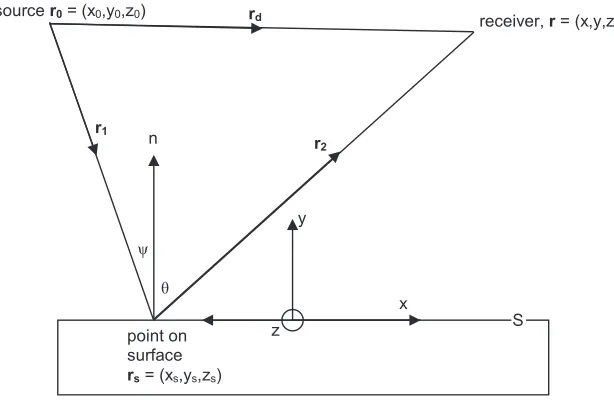
First, the formulation for non-absorbing, thin reflectors such as curved or flat surfaces is derived using the geometry shown in Fig. 1. The sound field at receiver point rand time t in the vicinity of a scatterer S is represented by the pressure ptðr;tÞ ¼piþps,

wherepi represents the sound traveling directly from the source to the receiver along

vector rd, andps the sound scattered off the surface. The pressure can be found from

the Kirchhoff integral equation3

ptðr;tÞ ¼piðr;tÞ þ

ðð

S

½ptðrs;tÞ ^n:rgðrjrs;tÞ gðrjrs;tÞ ^n:rptðrs;tÞds; (1)

wherersis a point on that surface; nis the normal to surface, anddenotes

gðrajrb;tÞ ¼

dðtRab=cÞ

4pRab

; (2)

whereRab ¼rarb anddðÞis a Dirac delta function. As the surface material is

consid-ered to be hard and non-absorbing, the last term in the integral in Eq.(1), which rep-resents the normal component of the particle velocity, is for now assumed to be zero. The incident field is taken to be created by a monopole with time-dependent ampli-tude,FðtÞ,

piðr;tÞ ¼FðtÞ gðrjr0;tÞ ¼Fðtrd=cÞ; (3)

where rd is the vector from the point source to the receiver point and c the speed of

sound.

For non-absorbing materials, the Kirchhoff boundary conditions simply states that there will be a doubling of the incident pressure at the surface,1i.e.,pt¼2pi and

^

n:rptðrs;tÞ ¼0. Learning from the frequency domain models that use this boundary

condition, it would be anticipated that inaccuracies will arise when the surface: (i) has significant corrugation that can then create second order reflections and (ii) is small compared to wavelength, because edge diffraction is not fully modeled.

To solve the integration, the surface is discretized into N elements that are small compared to wavelength, so the pressure can be approximated to be constant across the elements. Applying this to the integral equation with the source function and boundary condition gives

ptðr;tÞ ¼F tð Þ gðrjr0;tÞ þ2X

N

n¼1

cosðhÞ

ðð

F tð Þ gðrsjr0;tÞ

@gðrjrs;tÞ

@r2 ds; (4)

whereh is the angle of reflection relative to the surface differential normal andr2 the vector from the point on the surface to the receiver. The last term includes the differen-tial of the Green’s function, which is the differendifferen-tial of a delta function. This is dealt by using the following identity that exploits the quotient rule and includes a far field approximation so that the 1=r2 term can be moved outside the differential:4

Fig. 1. The geometry used in the prediction models.

F tð Þ @gðrjrs;tÞ @r2

1 4pr2c

_

F tr2

c

; (5)

where a dot over the function signifies the time derivative. Substituting Eq. (5) into Eq.(4)yields

ptðr;tÞ ¼F tð Þ gðrjr0;tÞ 2X

N

n¼1

cosðhÞ

4pr2c

ðð

gðrsjr0;tÞ F t_

r2 c

ds: (6)

As it has already been assumed that this is a far field model, the term in 1=r2 can be moved outside the integration. A Gaussian function is chosen as the excitation func-tion, as it is commonly used in many time-domain models5

F tð Þ ¼ _{ffiffiffiffiffiffi}1

2p p

re

_ðt2_=2r2_Þ

: (7)

The following differential is also required:

_

F tr2

c

¼

tr2

c

cr2 F t r2

c

: (8)

Substituting Eqs.(7)and(8)into Eq.(6)yields

ptðr;tÞ ¼

1 4pffiffiffi2p3=2_rrde

ðtrd=cÞ2=2r2

X

N

n¼1

cosðhÞ

8pffiffiffi2p5=2_r1r2r3_c

ðð

dðtr1=cÞ tr2

c

eðtr2=cÞ2=2r2ds; (9)

where 1=r1 has been moved outside the integration as this is a far field solution. The integration in Eq.(9)is treated as a simple summation and the convolution with the delta function is resolved. If each element has areaDs, then the pressure is

ptðr;tÞ ¼

1 4pffiffiffi2p3=2_rrde

ðtrd=cÞ2=2r2

X

N

n¼1

cosðhÞDs

8pffiffiffi2p5=2_r 1r2r3c

tr1þr2

c

eðtðr1þr2Þ=cÞ2=2r2: (10)

The plane and curved reflectors are assumed to be thin. The front face is discretized into elements that are smaller than a sixth of a wavelength for the highest frequency of interest. An important detail of note is that the accurate modeling of arrival times of the Gaussian pulses is vital and so oversampling is used.6Equation (10)is calculated with a sampling frequency at least ten times the highest frequency of interest and the samples of each Gaussian pulse are moved to the nearest sample point.

psðr;tÞ ¼ X

N

n¼1

cosðhÞDs

8pffiffiffi2p5=2_r 1r2r3c

t2dnþr1þr2

c

eðtð2dnþr1þr2Þ=cÞ 2

=2r2

: (11)

Equation (11) is equivalent to common models used in the frequency domain (e.g., Ref. 7) and will be described as the Fraunhofer model. This representation is expected to be suitable under similar conditions that the analogous frequency-domain model works: (i) the frequency content of the Gaussian pulse must be low enough that plane wave propagation in the wells dominates; (ii) the radiation coupling between the wells has to be small, and (iii) the radiation impedance of each well must be small.

A comparison of Eqs.(1) and(11)show, however, that the approximations in the derivation has removed some effects that arise for oblique incident sound, because there are no terms that explicitly have the angle of incidence,w. A more precise model needs to include the last term of Eq. (1). For this, the Kirchhoff Boundary condition also needs to be more completely considered. For a Schroeder diffuser, the pressure at the well entrance can be approximated as ptðr;tÞ ¼piðr;tÞ þpiðr;t2dn=cÞ. The first

term represents an incident wave traveling with an angle ofwto the normal. The sec-ond term is the wave reflected from the surface at an angle of w0 to the normal. Following the normal rules of refraction, for many surfaces, w0¼w would be an appropriate assumption. But for the narrow wells in a Schroeder diffuser, a better approximation might be that the reflected waves that reradiate from the wells travel parallel to the surface normal, w0¼0. Applying this to Eq. (1) and simplifying yields the following for the scattered pressure:

Fig. 2. Impulse response for (a) plane surface with both direct and reflected sound shown; (b) plane surface, reflection only; (c) curved surface, reflection only; (d) Schroeder diffuser, reflection only, Fraunhofer model; and (e) Schroeder diffuser, reflection only, Kirchhoff model. The peak of the direct sound has been set to unity for the plots. The insets in (c) and (d) illustrate two of the surface shapes.

psðr;tÞ ¼

Ds

16pffiffiffi2p5=2_r1r2cr3

X(

tr1þr2

c

eðtðr1þr2Þ=cÞ2_=2r2

cosð Þ h cosð Þw

þ tr1þr2þ2dn

c

eðtðr1þr2þ2dnÞ=cÞ2=2r2cosð Þ þh cos w0

)

: (12)

This will be referred to as theKirchhoff model, and is implemented in a similar manner to the previous models.

3. Validation

The results section include example predictions for various samples. The geometry cho-sen for the illustration were picked at random. The surfaces were all 1.41 m in size. The curved surface was such that the difference between the minimum and maximum corrugation was 19 cm. The shape of the corrugated surface was formed by adding some randomly chosen harmonics to create a wavy shape [see inset in Fig. 2(c)]. A one-dimensional quadratic residue diffuser was made based on the prime number 7 with the depth sequence along the x-direction. There were ten periods and the well width was 2 cm. The design frequency was 1000 Hz. The following (x,y,z) coordinates for the oblique source and receiver positions were chosen: (2.5, 4, 1) and (4, 3, 1) m, respectively. Predictions were carried out up to 8 kHz. A sampling frequency of 128 kHz was used and there were eight elements per minimum wavelength for the sur-face discretization.

To check that the new models were correct, the scattering was compared to standard single-frequency models. These are evaluations of the Helmholtz-Kirchhoff Integral Equation after the Kirchhoff boundary conditions had been applied. The fre-quency domain equivalent of Eqs.(10)and(11)is Eq. (8.26) from Ref.1with the sur-face reflection coefficientR(rs) explicitly stated as follows:

ptrÞ ¼Gðrjr0Þ ik

ðð

S

RðrsÞGðrsjr0ÞcosðhÞds; (13)

where k is the wavenumber and the frequency domain Green’s function is

GðrajrbÞ ¼expðikRabÞ=4pRab. The frequency domain equivalent of Eq. (12) for the

scattered pressure from a Schroeder diffuser is Eq. (8.25) from Ref.1,

psðrÞ ¼ ik

ðð

Gðrsjr0ÞGðrjrsÞ½ðcosðhÞ cosðwÞÞ þ ðcosðhÞ þcosðw0ÞÞRðrsÞds: (14)

4. Results

Figure2shows the pressure vs time for the three surfaces tested using the various time domain formulations. Figure 2(a) shows both the direct and reflected sound for the plane surface. Figures 2(b)–2(e) zoom in on just the scattered sound for: (b) plane, (c) curved, (d) Schroeder diffuser, Fraunhofer model, and (e) Schroeder diffuser, Kirchhoff model. For the plane surface, the reflection from the center of the surface and the additional delayed edge diffraction waves are as expected. The other surfaces create complex reflection patterns because of waves reflecting from different parts of the surface.

5. Conclusions

New formulations have been developed that allow the scattered impulse response from architectural surfaces such as reflectors and diffusers to be rapidly predicted. The meth-ods exploit the Kirchhoff boundary conditions and are analogous to a set of single-frequency models that are commonly used. The single-single-frequency models have been shown to be accurate for reflectors and diffusers with low absorption made from mate-rials such as hardwood, metal, and glass reinforced gypsum. The new methods are anticipated to work in the same situations with the advantage that they can more rap-idly obtain the impulse response.

FDTD models have a computational cost that scales with the maximum fre-quencyf atOðf4_{Þbecause of the combination of using a volumetric mesh and iterative}

time stepping. In contrast, the new time-domain models use a summation over a sur-face mesh with computation cost scaling at Oðf2_{Þ. Consequently, in many scenarios,}

the new models will be faster than FDTD methods. FDTD will be more accurate, however, because the Kirchhoff boundary conditions are only an approximation of the true surface pressure. The new approaches are intrinsically slower than geometric mod-els because accurate modeling of wave effects requires a higher spatial sampling than is normally used in geometric methods such as ray tracing. The new methods are inherently more accurate at modeling diffraction than geometric methods, however, because the new formulations are wave-based solutions. Example code for the predic-tion methods used to generate the figures can be downloaded from Ref.9.

Acknowledgments

Thanks to Jonathan Hargreaves for his invaluable comments on the method and paper.

References and links

1_{T. J. Cox and P. D’Antonio,Acoustic Absorbers and Diffusers(Taylor and Francis, London, 2009), pp.}

252–288.

2_{M. A. Heckl, “Numerical methods,” inModern Methods in Analytical Acoustics: Lecture Notes, edited by}

D. G. Crighton, A. P. Dowling, J. E. Ffowcs Williams, M. A. Heckl, and F. A. Leppington (Springer-Verlag, Berlin, 1992), pp. 283–310.

3

J. A. Hargreaves and T. J. Cox, “A transient boundary element method model of Schroeder diffuser scat-tering using well mouth impedance,” J. Acoust. Soc. Am.124, 2942–2951 (2008).

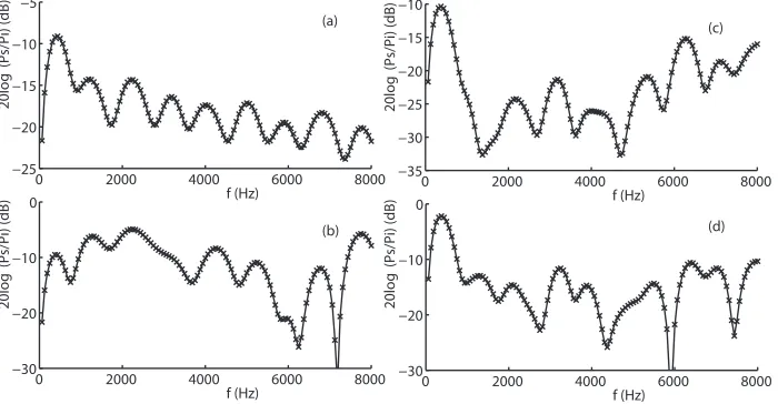
Fig. 3. Ratio of scattered to incident pressure in decibels for the time domain (solid line) and frequency domain models (). Surfaces: (a) plane; (b) curved; (c) Schroeder diffuser, Fraunhofer models Eqs.(11)and(13); and (d) Schroeder diffuser, Kirchhoff models Eqs.(12)and(14).

4

J. A. Hargreaves, “Time domain boundary element method for room acoustics,” Ph.D. thesis, University of Salford, Salford, UK, 2007, pp. 218. Available at http://usir.salford.ac.uk/16604/ (Last viewed February 5, 2015).

5

J. Sheaffer, M. van Walstijn, and B. M. Fazenda, “Physical and numerical constraints in source modeling for finite difference simulation of room acoustics,” J. Acoust. Soc. Am.135, 251–261 (2014).

6_{U. P. Svensson, R. I. Fred, and J. Vanderkooy, “An analytic secondary source model of edge diffraction}

impulse responses,” J. Acoust. Soc. Am.106, 2331–2334 (1999).

7

P. D’Antonio and J. H. Konnert, “The reflection phase grating diffusor: Design theory and application,” J. Audio Eng. Soc.32, 228–238 (1984).

8_{K. Kowalczyk, M. van Walstijn, and D. T. Murphy, “A phase grating approach to modeling surface}

dif-fusion in FDTD room acoustics simulations,” IEEE Trans. Audio Speech Language Processing19(5), 528–537 (2011).

9