ISSN: 1992-8645 www.jatit.org E-ISSN: 1817-3195
8352
THE STUDY OF NON-SAMPLED AREA IN THE SMALL
AREA ESTIMATION USING FAST HIERARCHICAL BAYES
METHOD
1KUSMAN SADIK, 2*ANANG KURNIA 3ANNASTASIA NIKA SUSANTI
1,2,3Department of Statistics, Faculty of Mathematics and Natural Science, Bogor Agricultural University
Jl. Raya Dramaga, Bogor, West Java INDONESIA 16680
E-mail: 1[email protected] , 2[email protected], 2[email protected] *Corresponding Author : [email protected]
ABSTRACT
Small area estimation is a method that arises as a result of the inability of direct estimator to provide an estimator with high precision when the sample size is inadequate. One of small area estimation methods which is widely used to estimate the poverty indicators is a hierarchical Bayes (HB). Yet, the used of HB method needs an intensive computation and requires a full census of covariates or auxiliary variables while in the fact this condition is difficult to reach. This paper proposed a method as the solution of this matter by using the fast hierarchical Bayes approach (FHB) to estimate the poverty indicators. Nevertheless the other problem arises when some of the areas have no sample unit. Therefore, this paper adding the use of cluster information to estimate the area effect. The simulation study is done in two conditions : (1) all the areas have sample units, (2) some areas have no sample units. The evaluation is based on Absolute Relative Bias (ARB) value, Relative Root Mean Square Error (RRMSE) value, and the computational time. Both of the simulation studies showing that the ARB and RRMSE of FHB and HB method is not significantly different. In terms of the computational time, FHB method consumes very less time than the HB method. Thus, it can be said that the FHB method is more effective to use than the HB method especially when the population size is very large. The application study is done to estimate the FGT poverty indicators of the sub-districs in Bogor Regency. The results show that the FHB method can provides better estimator of poverty indicators than the direct estimator, especially in the non-sampled area by adding the cluster information. It can be seen by the posterior variance of FHB estimator which provided very small variances.
Keywords: Cluster Information, Non-sampled Area, Fast Hierarchical Bayes,Small Area Estimation, Poverty Indicators
1. INTRODUCTION
The survey is a statistical method which is collecting the data by sampling the population. It provides an effective way to estimate the population characteristics [1] rather than collecting the data across the population. The sample size of the survey is frequently inadequate and it allows some area not surveyed [2]. Therefore the traditional area-specific direct estimators are not reliable since the area sample size is too small [3]. If the estimation of parameters solely based on the survey’s sample, then the estimator becomes inefficient because the estimator will have large variance [4]. The problem of small sample size,
even non sample area, can be solved by using the indirect estimation method that uses the model approach [2]. The statistical science that combines survey sampling, which has small sample sizes with statistical models is known as small area estimation [5]. The examples of small areas involve a geographical region, a demographic group, a demographic group within a geographic region, etc. [6]. This method is based on model usage, i.e. random effect models or mixed models [7].
8353 The availability of good auxiliary variables which can explain the variable of interest are very important in terms of small area estimation [10]. Small area estimators in most of the literature are also known as a composite estimator [11] which is the combination of the direct survey and the synthetic estimation [12]. Small area models are divided into two basic models [13]: (1) basic area level model that relates the direct estimators of small area into the covariate of a certain area since the auxiliary variables are unavailable at the unit level [14] ; (2) basic unit level model that relates the unit value of the variable of interest into the covariate value of a certain unit [15]. Area level model is widely used in the official statistics application by using the Fay-Herriot (FH) model [16] while the unit level model frequently uses the Nested Error Regression (NER) model proposed by [17,18]. The first unit level model was proposed by Elbers, Lanjow and Lanjow (ELL) to estimate the poverty indicators [19] which has been extensively used by the World Bank.
The application of small area estimation has been used in any fields such as in health, agriculture, income, and the most widely used is in the poverty mapping [20]. The problem of poverty is a problem that is often faced by almost all countries in the world. Therefore,it is important for the government to know the level of poverty even in the small region or subpopulation. The poverty rate can be measured in many different indicators. One of those is FGT (Foster, Greer, and Thornbecke) poverty measures [21]. The FGT poverty measures are based on the basic needs approach include the poverty incidence, poverty gap, and poverty severity which is calculated by comparing the welfare variable to the poverty line. The poverty mapping in a small area has been discussed by some researchers with different estimation methods. The methods that have been applied are the M-quantile models [22], the empirical Bayes [23], fast empirical Bayes [24], hierarchical Bayes [2], EBLUP with clustered information [25], and empirical Bayes with clustered information [26]. The study of small area estimation to estimate the FGT poverty measures by using the empirical Bayes [23] showed that the empirical Bayes provided best estimator since the Mean Square Error (MSE) value is small. Furthermore, the FGT poverty measures was estimated by using the hierarchical Bayes method by [2]. The study showed that both hierarchical Bayes and empirical Bayes approach practically give similar estimator based on the ARB and RRMSE value.
In the small area estimation, the possible problem that might be occured is non-sampled areas i.e. an area with unavailable sample units. Therefore, the area random effects of those areas cannot be estimated since no sample units are available. This paper proposed a solution of the problem by adding the cluster information. The estimation method that will be used in this paper is fast Hierarchical Bayes (FHB) as a new version of hierarchical Bayes (HB) method [2] since HB requires the full census of auxiliary variables of the units in the population.
This research focuses to solve the non-sampled area problem in terms of small area estimation since this problem is very possible to be happened. The estimation process is done by using the FHB method to estimate the FGT poverty indicators [26] since there is no research related to FHB method. The FHB can be implemented analogously to the fast EB (FEB) approach as in [24]. The FHB will be applied to the condition when all areas have the sample units and some areas of the survey are non-sampled. The estimator of FHB method will be compared with the HB method to see the performance of FHB method compared to HB method . The evaluation of estimators is based on the Absolute Relative Bias (ARB) and Relative Root Mean Square Error (RRMSE) value.
The organization of this paper is as follows. Section 2 describes the algorithm of forming posterior distribution as hierarchically. Section 3 presents the problem formulation in the research and how the FHB method works to estimate the poverty indicators. Section 4 provides the results and discussion by using simulation study and application study. Finally, in Section 5 give some concluding remarks of the research.
2. MATERIALS AND METHODS
The research is done first by using a simulation study with R software with the specification of the computers which have Intel Core i3 processor and 4 GB of Random Access Memory (RAM). Then, the research is applied to the real data to estimate the FGT poverty indicators. In this research, the FHB method that will be used to estimate the FGT poverty indicators is compared first with the HB estimator through the simulation study to see how well the FHB provides the estimators and how fast the computation time is.
ISSN: 1992-8645 www.jatit.org E-ISSN: 1817-3195
8354 population size and the sample size of each area are set variously with aimed to see the performance of the FHB method against the HB method. The population sizes that used are Nd1 = 1000, Nd2 = 5000, and Nd3 = 20000 and the sample sizes are nd1 = 5, nd2 = 10, and nd3 = 80. Yet, in the second condition the population area sizes that will be used is Nd3 = 20000 with the sample size as various as the first condition. The simulation is done with K =
100 times of sampling through the simple random sampling without replacement.
The application study of this research is aimed to estimate the FGT poverty indicators of all sub-districts in Bogor Regency as one of the poorest regency in West Java, Indonesia. The data is obtained from National Socio-Economic Survey (SUSENAS) by Central Bureau of Statistics of Indonesia (BPS) in 2013 while the auxiliary variables is obtained by Village Potential Survey (PODES) in 2014. The unit study of this application study is the household and the variable of interest is per capita expenditure. There are six auxiliary variables that used in this study as in [26]:
1) The proportion of village with the main source of income is in the agriculture
2) The proportion of the number of village with the main source of income is in the processing industry.
3) The proportion of the number of village with the main source of income is in the large trade or retail and restaurants.
4) The proportion of the number of village with the main source of income is in the service sector.
5) The proportion of grocery stores. 6) The proportion of restaurants .
The difficulty of Bayes method is to specify the prior because it can influence the posterior distribution. The selection of incorrect prior can obtain an improper posterior which is not integrated into one. Then, based on [2], the Jeffrey prior is a great choice since it is a noninformative prior and it is the square root of Fisher Information. As described in [2], the use of Markov Chain Monte Carlo (MCMC) method for HB is avoided. This is caused by a very long computation time since the MCMC method need the monitoring of the Markov Chains for each generated sample to be convergence. Then it needs a reparameterization in the form of intra-class correlation as in [2] by ρ= δ2/( δ2 + σ2) to avoid the used of MCMC method. Based on [2], the posterior distribution can be formed by:
π(u, β, σ2, ρ|y
s) = π1(u| β, σ2, ρ, ys) π2(β| σ2, ρ, ys) π3(σ2 |ρ, ys) π4(ρ| ys) (1)
The posterior distribution in (1) can be obtained by following the steps as described in [26]:
1. Generated the population with the auxiliary variables i.e x1~binom(Nd, p=0.3+0.5 x d/D) and
x2~binom(Nd, p=0.2), the coefficient regression
β is (3, 0.03, -0.04)’, the area random effects variance σ2u = 0.152, and the error variance σ2 = 0.52 through the NER model :
ydi = x’di β + ud + edi (2)
with d = 1, 2,...,D; i=1,2,...,Nd, xdi is the px1 vector of auxiliary variable, β is the px1 vector of regression coefficients, ud is a random effect of area d which is iid distributed as ud|σ2~N(0,σu2), and edi is errors which is iid distributed as edi|σ2~N(0,σ2wdi-1) with wdi >0 is heteroscedasticity weight.
2. Calculated the parameters of area d =1,2,...,D of
FGT poverty indicators by
Pαd = 1 /Nd
Nd
i1
Pαdi ; i = 1,2,...,Nd (3)
Pαdi =[ ( z- Edi) / z]αI(Edi < z) ; α = 0,1,2 (4)
Edi is inverse transformation of ydi ; z is poverty line which is obtained by 0.6 x median of Edi [2]; α shows the poverty indicators i.e α =0 is Poverty Incidence (P0), α =1 is Poverty Gap (P1), and α=2 is Poverty Severity (P2) with the
indicator function : I(Edi < z) = 1 if Edi < z (poor) and I(Edi < z) = 0 if Edi > z (not poor) 3. Draw nd samples from each area then the direct
estimators can be obtained by
Pαd = 1 /nd
nd
i1
Pαdi , d= 1,2,...,D (5)
4. Generated the posterior distribution in equation (5) by following steps :
4.1.Generated the distribution of ρ by making a grid of R = 1000 then the π4(ρ| ys) can be written as
π4(ρr) = k4(ρr) /
R
r 1
k4(ρr) (6)
with
8355 [γ(ρr)]-(n-p)/2
*
1
D
d
λd1/2(ρr); r=1,2,...,R-1
wd.=
sd iwdi
in this study the wdi is assumed equal to 1.
λd (ρ) = wd. [wd. + (1- ρ/ ρ)]-1
xd = 1 / wd. [
sd iwdi xdi ] and
yd = 1/wd. [
sd iwdi ydi ]
Q(ρ) =
*
1
D
d
isdwdi (xdi - x)(xdi - x)’ +
1-ρ/ρ
* 1 D dλdxdxd’
p(ρ) =
*
1
D
d
isdwdi (xdi - x)(Ydi - y)’ +
1-ρ/ρ
* 1 D dλdxdyd
ˆ
(ρ) = Q-1 (ρ) p(ρ) γ (ρ) =
*
1
D
d i
sdwdi [(Ydi - yd - )
(xdi - x)’
ˆ
(ρ)]24.2.Generated ρ as much H by discrete
distribution { ρr , π4(ρr )}then add it to the H uniform distribution in the interval (0, 1/R). 5.Generated the error variance distribution from
π3(σ2 |ρ, ys) distribution
σ -2 |ρ, y
s ~Gamma ( (n –p)/2, γ (ρ)/2) (7)
Then take = 1/ σ -2.
6.Generated the π2(β| σ2, ρ, ys) distribution i.e
β| σ2, ρ, y
s ~ N (
ˆ
(ρ), σ2(Q)-1(ρ)) (8) 7.Generated the area random effects fromud| β ,σ2, ρ, ys ~ N [λd (ρ) (yd - xd’ β) , (1- λd (ρ))
σ2 ρ/1- ρ] (9)
8.Finally the posterior distribution of π(u, β, σ2, ρ|ys) is described as
Ydi|ys, θ ~ N(xdi’ β + ud , σ2) (10)
Based on the posterior distribution in equation (10) then the FHB and HB estimators of FGT poverty measures can be calculated. Those estimators can be obtained by using the Monte Carlo approximation since the posterior distribution π(u, β, σ2, ρ|y
s) is very complex. The Monte Carlo process is started from step 5 to step 8 as much as Monte Carlo repetitions. In this study, we use H =
100of Monte Carlo. Then FGT estimators can be obtained by calculating the posterior means in each Monte Carlo repetitions. Furthermore, by averaging the FGT estimators for each Monte Carlo, then it will be obtained the FGT estimator for one sampling. This process is repeated as much as K =
100 times of sampling.
3. PROBLEM FORMULATION AND SOLUTION
The possible problem in the small area estimation is a non-sampled area. Then, the area random effects can not be estimated. This research give an alternative way to solved the problem by adding the cluster information to subtitute the area random effects on non-sampled area using the FHB method. Based on the Section 2, after the posterior distribution was formed, then the FHB estimation can be conducted. The FHB estimators can be obtained by following the steps:
1. Clustering all areas by using the Ward method based on the previous research by [27] to see the non-sampled areas lied on which cluster.
2. The area random effects of the non-sampled areas are estimated by averaging the λd, yd, and xd then generated the area random effects of non –sampled areas based on equation (9).
3. Generated the variable of interest based on (10) as much of the original sample size and repeat
H times over the Monte Carlo. Then calculated
the FHB estimator of the poverty indicators by:
ˆ
dFHB =P
ˆ
αdFHB = E(δd|ys)≈ 1/H
H
h 1
ˆ
d(h)≈ 1/H
H
h 1
P
ˆ
αd(h) (11)ISSN: 1992-8645 www.jatit.org E-ISSN: 1817-3195
8356 for HB method as much of Nd - nd then combines with the variable of interest of sample units. The HB estimator of the poverty indicators can be calculated from H times
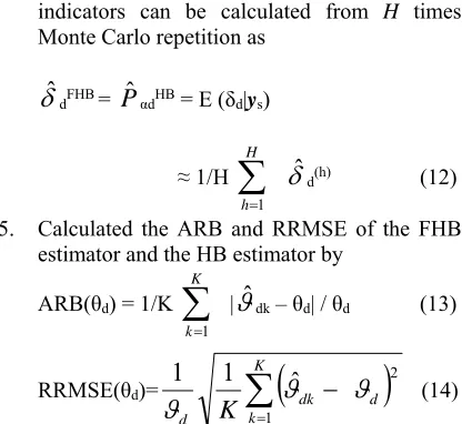
Monte Carlo repetition as
ˆ
dFHB =P
ˆ
αdHB = E (δd|ys)≈ 1/H
H
h 1
ˆ
d(h) (12)5. Calculated the ARB and RRMSE of the FHB estimator and the HB estimator by
ARB(θd) = 1/K
K
k 1
|
ˆ
dk – θd| / θd (13)RRMSE(θd)=
K
k
d dk
d
K
12
ˆ
1
1
(14)Then compared the ARB and RRMSE values of FHB and HB method.
4. RESULTS AND DISCUSSION
4.1. Simulation Study
The first study in this research is simulation study to see the performance of FHB method. Then, in the simulation study, there are two setting conditon, i.e when all areas have sample unit and some areas are not surveyed. The results of those simulations are provided as follows.
4.1.1. All areas have sample unit
[image:5.612.91.299.129.320.2]The simulation study of this condition is basically done to see how well the performance of the FHB method to estimate the poverty indicators. Its performance is seen from various sides such as the sample sizes, the population area sizes, and the computational time with the goodness of the performance is measured by the ARB and RRMSE value. The results of the sample size effects are presented in Table 1.
Table : 1 The ARB and RRMSE Value of Poverty Indicators by Using Various Sample Sizes.
Indicators Sample Sizes ARB RRMSE
Computation Times (Minutes) Direct
Estimator HB FHB Estimator Direct HB FHB HB FHB
P0
5 0.912 0.397 0.410 1.099 0.480 0.503 59.28 8.60 10 0.630 0.329 0.334 0.782 0.400 0.408 60.01 8.82 80 0.213 0.137 0.139 0.267 0.172 0.174 63.75 10.94
P1
5 1.078 0.548 0.566 1.395 0.675 0.706 59.28 8.60 10 0.789 0.484 0.451 0.999 0.546 0.559 60.01 8.82 80 0.272 0.173 0.177 0.341 0.218 0.222 63.75 10.94
P2
5 1.248 0.694 0.718 1.842 0.868 0.916 59.28 8.60 10 0.984 0.551 0.563 1.344 0.685 0.708 60.01 8.82 80 0.364 0.206 0.212 0.457 0.260 0.267 63.75 10.94
Table 1 shows that the increasing in the number of sample sizes resulted in the ARB and RRMSE values which is obtained by the direct estimation, HB, and FHB method becoming smaller. Based on the table, it can be seen that the smallest ARB and RRMSE value is resulted by HB method while the FHB method has a little bigger of those values. The relative efficiency of FHB method against the HB method based on the ARB and RRMSE value is bigger than one. It means that HB is more efficient than the FHB method. However the difference between ARB and RRMSE
values generated by HB and FHB method is very small.
[image:5.612.112.526.402.568.2]8357 The result is presented in Table 2.
Table 2 :The ARB and RRMSE Value of Poverty Indicators by Using Various Population Area Sizes.
Population Area Sizes
Indicators ARB RRMSE
Computation Time (minutes) Direct
Estimator HB FHB Estimator Direct HB FHB HB FHB
Nd1 = 1000
P0 0.592 0.329 0.334 0.730 0.399 0.408
14.83 8.99
P1 0.716 0.463 0.472 0.931 0.568 0.585 P2 0.867 0.600 0.614 1.238 0.741 0.771
Nd2 = 5000
P0 0.582 0.287 0.294 0.708 0.352 0.363
28.24 9.15
P1 0.714 0.382 0.392 0.909 0.476 0.492 P2 0.862 0.472 0.486 1.208 0.595 0.620
Nd3 = 20000
P0 0.581 0.247 0.255 0.710 0.301 0.314
139.98 10.22
P1 0.708 0.297 0.329 0.895 0.395 0.411 P2 0.867 0.379 0.393 1.197 0.476 0.500
Table 2 shows that the increasing of population area sizes generally causes the ARB and RRMSE value of each poverty indicators getting smaller. Based on the table, it can be seen that the value of ARB and RRMSE which is obtained by the FHB method and the HB method is not too be different. Table 2 also shows the computational time which both HB method and FHB method needed to run the program for all population area sizes. It can be seen that the increasing of population area sizes causes the longer computation time.
Based on the table, when the population size is large, the HB method needs too much time of computation and it makes the HB is not effective to use since the HB method needs computation time about 13 times of FHB computation time. Therefore, the FHB method is an appropriate method of estimation when the population size is very large since the FHB practically gives the similar ARB and RRMSE value as HB method.
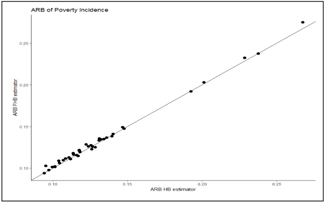
The figures below show the ARB and RRMSE value of each area of the Poverty Incidence as an example.
[image:6.612.153.479.513.715.2]ISSN: 1992-8645 www.jatit.org E-ISSN: 1817-3195
[image:7.612.105.476.63.324.2]8358
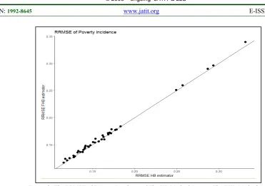
Figure 2: The RRMSE of Poverty Incidence of The HB Method Against The FHB Method
.
Based on the Figure 1 and Figure 2, it can be seen that the ARB and RRMSE value of the HB and the FHB method is practically similar since both of them lied on the straight line even though in some areas the ARB and RRMSE value of FHB is a little bigger than HB. Yet it can be said that both HB and FHB are giving a good estimator.
4.1.2. Some non-sampled areas
The simulation study of this condition is aimed to see the performance of FHB method when some areas of the survey are non-sampled. Therefore, in those areas the sample units are unavailable then the direct estimation of those areas can be calculated. Therefore, this study uses the cluster information of the non-sampled area to subtitute the random area effect by using the FHB method. Then, it will be compared the result of FHB method with the HB method to see the performance of FHB method to give the estimator when the sample units are unavailable. The result is presented in Table 3.
Table 3 :The ARB and RRMSE value of poverty indicators in the non-sampled area using the FHB method
Area Indicators Parameters Estimators ARB RRMSE
HB FHB HB FHB HB FHB
16
P0 0.2074 0.2205 0.2204 0.0636 0.0635 0.0718 0.0717 P1 0.0516 0.0683 0.0683 0.3227 0.3223 0.3273 0.3270 P2 0.0186 0.0300 0.0300 0.6120 0.6115 0.6172 0.6167
21
P0 0.2360 0.2204 0.2204 0.0661 0.0663 0.0723 0.0725 P1 0.0603 0.0683 0.0682 0.1322 0.1317 0.1403 0.1399 P2 0.0223 0.0300 0.0300 0.3421 0.3414 0.3485 0.3478
40
[image:7.612.106.509.538.720.2]8359 Table 3 shows that the addition of cluster information causes the estimating process can be done in non-sampled area while the direct estimation is unavailable. Based on the table, both HB and FHB practically give the similar estimator in each non-sampled area. It is also supported by the ARB and RRMSE values of those methods which give the similar value. The simulation in the first condition, which is all areas have sample units, shows that the FHB method is more effective and faster in the computation time than the HB method. Therefore, FHB is more appropriate to use when the population size is very large. Then in the simulation study use the FHB method to estimate the FGT poverty indicators.
4.2. Application Study
The application study of this research is applied on Bogor Regency data to estimate the FGT poverty indicators in its sub-districts in 2013. First, the data is explored to the purpose of knowing the characteristics of the data. Based on the results of exploration data, it is known that Bogor Regency is consist of 40 sub-districts. Moreover, there are three subdistrics in Bogor Regency data of National Socio-Economic Survey in 2013 that are non– sampled. The non-sampled areas are Megamendung sub-district, Tanjungsari sub-district, and Parung Panjang sub-district. Then the data is appropriate to applied the proposed method of this research.
Based on the Village Potential Survey (PODES) data in 2014, the sub-districts of Bogor Regency is clustered by using the auxiliary variables as mention in the Section 2. Then there are three clusters, i.e. (i) the first cluster with the number of member is 21 areas, (ii) the second cluster with the number of member is 11 areas, and (iii) the third cluster with the number of member is 8 areas.
It is known from the clustering method that all non-sampled areas are lied on the first cluster . It means that they will have the same area random effects since they have the similar characteristics of area.
The area random effects of non-sampled area are generated as in equation (9) with the mean obtained by averaging the
𝜆
,
𝑥
̅,d a n y̅
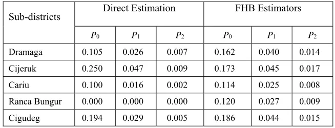
from other areas in the same cluster with the non-sampled area. Then the estimation of FGT poverty indicators can be done even in the non-sampled areas. Based on the data from Central Bureau of Statistics (BPS) of Indonesia, it is known that the poverty line in Bogor Regency in 2013 is Rp 252 542.00. A household is classified as poor people when its expenditure is below the poverty line. Otherwise, if the expenditure of a household is above the poverty line then it not classified as poor people. In this application study, the estimators of the direct estimation is compared with the estimator of the FHB method. The Table 4 below shows the FGT estimators for some sub-districs as an example. [image:8.612.142.469.578.703.2]Table 4 shows that both the method provide a significant difference of the FGT poverty estimators on some sub-districts. Yet, by using direct estimation, it is very possible to find that some sub-disricts have zero FGT poverty estimators where in the fact it is quite impossible. Then, by using the FHB method to estimate the FGT poverty indicators, all sub-districts that have the sample units have a non-zero FGT povety estimators. It makes more sense than the result from the direct estimation. This fact can be strengthened by the result of simulation study in both condition which shows that the FHB method provide better estimators than the direct estimation in terms of ARB and RRMSE value.
Table 4 : The Estimators of FGT Poverty Indicators on Some Sub-District in Bogor Regency
Sub-districts Direct Estimation FHB Estimators
ISSN: 1992-8645 www.jatit.org E-ISSN: 1817-3195
[image:9.612.89.301.204.314.2]8360 Based on the estimating process, it is also obtained the FGT poverty indicators of the non-sampled areas through the addition of the cluster information. The estimation of the FGT poverty indicators on the non-sampled areas are presented in Table 5 below.
Table 5 : The Estimators of FGT Poverty Indicators on The Non-Sampled Area
Sub-districts
Estimators of Poverty Indicators Poverty
Incidence (P0)
Poverty Gap (P1)
Poverty Severity
(P2) Megamendung 0.070 0.014 0.004 Tanjungsari 0.090 0.018 0.006 Parung Panjang 0.071 0.014 0.004
Table 5 gives the estimators of FGT poverty indicators on non-sampled area. It can be seen from the table that the FGT estimators in these areas are not different sigificantly. Based on the result, it is known that Tanjungsari sub-districts is the sub-districts with the highest Poverty Incidence between Megamendung and Parung Panjang sub-districts.
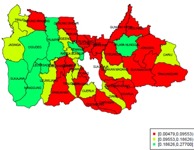
The distribution of the Poverty Incidence of all sub-districts in the Bogor Regency is provided in the Figure 3. The green areas show that those areas have high percentage of poor people. Then the yellow areas show that those area have the percentage of poor people lower than the green areas and the red areas show that those areas are the lowest percentage of poor people. Based on the estimation by using the FHB method, it can be known that Leuwisadeng sub-districts is the poorest sub-district in Bogor Regency since it has the highest percentage of poor people (Poverty Incidence) .Then Gunung Putri subdistricts is the richest sub-districs since it has the lowest all poverty indicators. It is in line with the fact that Gunung Putri has the highest per capita expenditure based on the SUSENAS data.
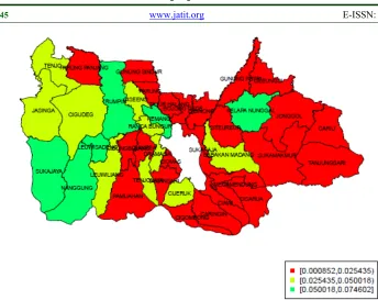
[image:9.612.152.474.424.673.2]Then the distribution of the Poverty Gap and Poverty Severity based on the FHB method is povided on the Figure 4 and Figure 5 respectively. The figures show that Bogor western past has higher Poverty Gap and Poverty Severity Indicators than Bogor in the middle and eastern part . Based on the FHB estimators, it can be known that Nanggung subdistricts has the highest Poverty Gap and Poverty Severity indicators while Gunung Putri sub-districts has the lowest Poverty Gap and Poverty Severity indicators.
8361
Figure 4: The Distribution of The Poverty Gap in The Bogor Regency
[image:10.612.193.501.391.591.2]ISSN: 1992-8645 www.jatit.org E-ISSN: 1817-3195
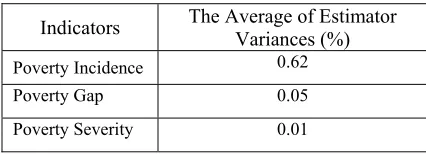
[image:11.612.89.302.219.296.2]8362 In the HB and FHB method, the goodness of the estimators can be measured directly by its posterior variances. It is because the inferentia of the HB and FHB is direct. That is, after the posterior distribution is formed, it can be used for all inferences. Based on the these, the average variance of the estimators is provided in Table 6.
Table 6 :The Average Variance of The estimators of FGT Poverty Indicators
Indicators The Average of Estimator Variances (%)
Poverty Incidence 0.62
Poverty Gap 0.05
Poverty Severity 0.01
Based on the Table 6, it can be known that the average variance of the FGT estimators by H = 100 times of Monte Carlo replications is less than 1 %. The small variance values indicate that the resulting estimates are consistent. Thus, it can be concluded that the estimator value based on the FHB method are reliable and better than direct estimation since the direct estimation enable zero value of the FGT estimator and it can provide the estimator in the non-sampled area.
4.3. Discussion
The small area estimation is an appropriate method to estimate the parameters when the sample size of a survey is too small. In addition, when there are some non-sampled area in a survey, the small area estimation can be used by adding the cluster information to substitute the missing area random effect of those areas. Yet in the small area estimation, the existance of auxiliary variables is a must since the information of the area target from the survey is inadequate.
The simulation study, both on the first simulation or the second simulation, shows that the HB method and the FHB method practically give the same value of ARB and RRMSE even though
the FHB gives a little bigger value. Therefore, it can be said that the FHB loses its efficiency since its RRMSE is bigger than HB. Yet the FHB is much better to use than the direct estimator in terms of ARB and RRMSE value. Furthermore, in terms of computational times, the FHB method takes less time than the HB method. It can be said that the FHB is more effective to use than the HB method. Hence, when the population target is very large then the FHB method is an appropriate method to use to estimate the parameters.
The application study shows that the Bogor western parts are consist of the sub-districts with high percentage of poor population. Then, the eastern part of Bogor and the middle part of Bogor generally have the low and medium poverty incidence. The FHB estimators of poverty incidence for all sub-districts is compared with the direct estimators which is obtained from the SUSENAS data. Then the average of both method is compared with the BPS publication of the Poverty Incidence in 2013 in the Bogor Regency. The BPS publication provides that the Poverty Incidence or percentage of poor people in Bogor Regency in 2013 is 8.83%. This value is lower than the weighted average based on the estimation with the FHB method, which is 8.92%. However, based on direct estimation, which are only based on the sample data, the weighted average value of the percentage of poor people in Bogor Regency is only 3.69%. It is caused since the direct estimation can not give the estimators in the non-sampled areas and since there are some areas which zero FGT poverty estimators. Then, by the results it can be known that the FHB provides the estimators more close with the BPS publication than the direct estimators.
This research has some limitations in estimating the FGT poverty indicators. The limitations include the effect time and the spatial effect since these characteristics are not considered in this research. Then a model with additional time effect and/or spatial correlation among the areas might be considered in the future research.
5. CONCLUSION
Based on the simulation study, even in the first condition and the second condition, it can be concluded that the HB method and the FHB method practically give the same ARB value even though the ARB value of FHB is a little bigger than HB method and so is the RRMSE value. Moreover, the addition of the cluster information in the non-sampled area can give better estimator than the direct estimation which can not provide the estimator. Nevertheless, in terms of computation time, the FHB is more effective than HB method. Thus the FHB method is appropriate to use when the population sized is very large
8363
ACKNOWLEDGEMENTS
This research is supported by the Indonesia Endowment Fund for Education (LPDP) which becomes as sponsorship of the author’s study and research.
REFRENCES:
[1]. S. Marchetti,N. Tzavidis,and M. Pratesi, “Non-parametric Bootstrap Mean Squared Error Estimation for M-quantile Estimators of Small Area Averages, Quantiles and Poverty Indicators”, Computational Statistics and Data Analysis,Vol. 56,No.10, 2012,pp. 2889–
2902.
[2]. I. Molina, B. Nandram, and J.N.K Rao,”Small Area Estimation of General Parameters with Application to Poverty Indicators: A Hierarchical Bayes Approach”, The Annals of Applied Statistics. Vol.8,No.2,2014,pp.
852-885.
[3]. F. Verret, J.N.K. Rao and M. A. Hidiroglou,” Model-based Small Area Estimation under Informative Sampling”,Survey Methodology,
Vol.41, No.2, 2015,pp. 333-347.
[4]. K. Sadik, “Metode Prediksi Tak-bias Linear Terbaik dan Bayes Berhirarki untuk Pendugaan Area Kecil Berdasarkan Model State Space”. Jurnal Forum Statistika dan Komputasi. Vol.15,No.2,2009,pp.8-13.
[5]. D. Morales, M.C. Pagliarilla, and R. Salvatore, “Small Area Estimation of Poverty Indicators under Partitioned Area-level Time Models”.SORT. Vol.39,No. 1, 2015, pp.
19-34.
[6]. J.Jiang, P. Lahiri. And T. Nguyen,“A Unified
Monte-Carlo Jackknife for Small Area Estimation after Model Selection”,Preprint, 2016, Available : arXiv:1602.05238.
[7]. J. Jiang and P. Lahiri, “Mixed Model Prediction and Small Area Estimation”.
Sociedad de Estad stica n Operativa.Vol.15,
No.1, 2006,pp. 1-96.
[8]. M. Ghos and J.N.K Rao,”Small Area Estimation : An Appraisal”. Statistical Science.Vol. 9,No. 1, 1994,pp. 55 -76.
[9]. A. Kurnia,”Prediksi Terbaik Empirik untuk Model Transformasi Logaritma di dalam Pendugaan Area Kecil dengan Penerapan pada Data Susenas”.Unpublished doctoral dissertation, Department of Statistics
FMIPA-IPB, Indonesia, 2009.
[10].J.N.K. Rao,” Small area estimation”. Small area models (pp: 75-76), 2003, New York (US): John Wiley and Sons.
[11].M.R. Ferrante and S. Pacei, “Small Area Estimation for Longitudinal Surveys”,
Statistical Methods & Applications, Vol.13,
No. 3, 2004,pp. 327-340
[12]. J. Jiang, “Empirical Best Prediction for Small-area Inference Based on Generalized Linear Mixed Models”, Journal of Statistical Planning and Inference , Vol. 111,2003,pp.
117 – 127
[13].M. Torabi,G.D. Datta, and J.N.K. Rao,
“Empirical Bayes Estimation of Small Area Means under A Nested Error Linear Regression Model with Measurement Errors in The Covariates”, Scandinavian Journal of Statistics, Vol. 36, No.2, 2009,pp. 355 – 369.
[14].Y. Marhuenda, I. Molina, and D. Morales, “Small Area Estimation with Spatio Temporal Fay-Herriot Models”. Computational Statistics and Data Analysis.Vol. 58,2013,pp.
308-325
[15].R. Chambers and N. Tzavidis, “M-quantile Models for Small Area Estimation”.
Biometrika. Vol. 93, No. 2, 2006, pp.
255-268.
[16].R.E. Fay and R.A. Herriot,” Estimates of Income for Small Places: An Application of James-Stein Procedures to Census Data”,
Journal of American Statistical Association,Vol. 74,No.366, 1979,pp.
269-277.
[17].G. E. Battese,R. M. Harter, and W. A. Fuller, “An Error Components Model for Prediction of County Crop Area using Survey and Satellite Data”. J. Amer. Statist. Assoc.Vol.
83, No. 401, 1988,pp. 28–36.
[18].N.G.N. Prasad and J.N.K Rao,”The Estimation of Mean Squared Error of Small Area Estimators”. J. Amer. Statist. Assoc.Vol.
85, No. 409,1990, pp.163–171.
[19].C. Elbers ,J. Lanjouw and P. Lanjouw, “Micro-level estimation of poverty and inequality” , Econometrica, Vol.71,No.1,
2003,pp. 355-364.
[20].J.N.K Rao and I. Molina,” Small Area Estimation”.2nd ed. ,2015, New York(US): John Wiley and Sons.
[21].J. Foster, J. Greer, and E. Thorbecke, “A Class of Decomposable PovertyMeasures”. Econometrica: Journal of the Econometric Society, Vol. 52, No.3, 1984, pp.761-766.
ISSN: 1992-8645 www.jatit.org E-ISSN: 1817-3195
8364 Application to Poverty Mapping”, Stat Meth Appl,Vol.17,2008,pp. 393 – 411.
[23].I. Molina and J.N.K. Rao,”Small Area Estimation of Poverty Indicators”,The Canadian Journal of Statistics,Vol. 38,
No.3,2010,pp. 369 – 385
[24].C. Ferreti and I. Molina, “Fast EB Method for Estimating Complex Poverty Indicators in Large Population”. Journal of The Indian Society of Agricultural Statistics,Vol 66, No.
1, 2012, pp.105 -120.
[25].R. Anisa,A. Kurnia, and Indahwati,“Cluster Information of Non-sampled Area in Small Area Estimation”, IOSR Journal of Mathematics (IOSR-JM). Vol.10, No. 1,
2014,pp. 15-19.
[26].V.Y. Sundara, K.Sadik, and A. Kurnia,. “Cluster Information of Non-sampled Area in Small Area Estimation of Poverty Indicators using Empirical Bayes”, AIP Conference Proceedings ,Vol.1827, No.1, 2017.