5464
EMPIRICAL STUDY ON BANDWIDTH OPTIMIZATION
FOR KERNEL PCA IN THE K-MEANS CLUSTERING
OF NON-LINEARLY SEPARABLE DATA
1CORI PITOY, 2SUBANAR, 3ABDURAKHMAN
1Mathematics Science Doctoral Program, Faculty of Mathematics and Natural Science, Universitas Gadjah Mada
2Department of Mathematics, Faculty of Mathematics and Natural Science, Universitas Gadjah Mada
E-mail : 1cori.pitoy@mail.ugm.ac.id, 2subanar@ugm.co.id, 3rachmanstat@ugm.ac.id
ABSTRACT
K-Means is a method of non-hierarchical data clustering, which partitions observations into k clusters so that observations with the same characteristics are grouped into the same cluster, while observations with different characteristics are grouped into other cluster. The advantages of this method are easy to apply, simple, and efficient, and its success has been proven empirically. The problem is when the data is non-linearly separable. Overcoming the problem of non-non-linearly separable data can be done through a data extraction and dimension reduction using Kernel Principal Component Analysis (KPCA). The results of KPCA transformation were affected by the kernel type and the size of bandwidth parameters (), as a smoothing parameter. Calculation of K-Means clustering of Iris dataset, using 2 Principal Component (PC), Euclid distance and Gaussian kernel showed that the external validity (entropy) and internal validity (Sum Square Within) are better than the result of standard K-Means algorithm.
Keywords: K-Means Clustering, KPCA Bandwidth, Validity, Entropy, Non-Linear Separable Dataset
1. INTRODUCTION
K-Means introduced by [1], attempts to find
k clusters so that observations with the same characteristics are grouped into the same cluster, while observations with different characteristics are grouped into other cluster. Assessment of the results of K-Means clustering algorithm is performed by using validity index. In general, the validity of the index is classified as the external and internal index as well as the relative index.
External indexes are used to measure the extent to which cluster labels match with an externally supplied class label usually expressed as the entropy, which evaluates the "purity" of cluster label based on the given class. The Internal indexes are used to measure the goodness based on clustering structure of data intrinsic information but not connected with external information. The function of internal criteria focuses on the observations of each cluster and does not take into account the observations of different clusters. The measurements include the value of SSW cluster [2].
The excellence of K-Means method is easy to be implemented, simple, efficient, and empirical
success. However, this method does not guarantee that the result of clustering is unique because it is sensitive to the selection of initial seeds. Initial centroid for K-Means clustering are randomly determined, thereby clustering the same data can produce different clusters [3]. K-Means clustering would work perfectly if clusters are linearly separable and spherical in shape. Meanwhile, the K-Means clustering performance is greatly affected when high-dimensional datasets are used [3]. This is due to the fact that data with a higher dimension has observations that are not linear in structure.
5465 Scholkopf et al. in [5] conducted a data extraction and dimension reduction using KPCA. The results of this extraction were affected by the kernel type and the size of bandwidth () used, which further affected the results of clustering. The size of bandwidth can also be determined subjectively or based on research that has been done before [6]. Therefore, the question in this researh is how the size of KPCA bandwidth that ensures the K-Means clustering of non-linearly separable data has high internal and external validation.
The motivation in this research is to study the superiority of K-Means clustering, which is obtained through KPCA transformation, compared to conventional K-Means. Furthermore, the K-Means clustering validation of the KPCA transformation result is performed by using SSW(%) and Entropy towards original and standard data. This calculation, which uses 1, 2 and 3 PCs, can be compared using bandwidth = 0.2 and = 0.3.
The article is organized as follows. Background is presented in Section 2, KPCA is detailed in Section 3, Simulations on real data set are presented in Section 4, Results and discussion are detailed in Section 5. Finally, Conclusion and Recommendation are drawn in Section 6.
2. BACKGROUND
KPCA is an extension of the non-linear PCA which is done through dimensional data reduction. The use of KPCA was introduced by [7] where the training data is mapped into high-dimensional feature space including even infinite dimensions. In this space, KPCA extracts the main components of the data distribution. For non-linearly separable cluster, [8] used the Kernel K-Means which is the development of a standard K-Means clustering algorithm. Two main advantages of this method are the deterministic factor which makes it independent of the cluster initialization and the ability to identify groups that non-linearly separable in the input space.
Chang [9] in his research, concluded that the Gaussian kernel is sensitive to the width of the kernel. Small bandwidth size will lead to over-fitting, otherwise the size of large bandwidth leads to under-fitting. Therefore, optimal kernel width has only been based on the tradeoff between the under-fitting loss and over-fitting loss. Thus, there is an urgent need to reduce the loss tradeoff.
In his research on SVC, [10] stated that the kernel width depends on the spatial characteristics of the data but does not depend on the amount of data or the dimensions of the dataset. A major challenge in SVC is a selection of parameter values, i.e. the width of the kernel function that determines the non-linear transformation of the input data. Serious weakness of kernel method is the difficulty in choosing the kernel function that is suitable for the dataset. No specific kernel function has the best generalization performance for all types of the problem domain and it suggests the combinations of various types of kernels to solve problems in Support Vector Machines (SVM). Chen et al. in [11] proposed the use of KPCA for SVM in feature extraction. Compared with other predictors, this model has a greater general ability and higher accuracy.
Furthermore, [12] using multiple bandwidth measures in his research, he trained the data with the SVDD algorithm for different values of from range 0.0001 to 8.0 by increment 0.05 and concluded that a spherical data boundary led to underfitting, while an extremely wiggly data boundary led to overfitting. At = 0.1, each point in the data was identified as a support vector, representing a very wiggly boundary around the data. As the value of increased from 0.1 to 0.6, the data boundary was still wiggly, with many “inside” points identified as the support vectors (SVs). As increased from 0.7 to 1.0, the boundary began to form the Banana shape.
So far, some of tested the sizes by [12] are related to the number of SVs and shapes of the cluster, but not discussing about the validity of clustering results. Therefore, in this research we will look for the size of the KPCA bandwidth that gives the K-Means clustering results in the feature space with high internal and external validation for the non-linear separable data.
3. KERNEL PRINCIPAL COMPONENT ANALYSIS (KPCA)
3.1.Kernel Trick
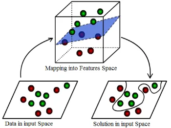
K-Means is an unsupervised clustering method that reallocates observations to each cluster, where an observation is explicitly stated as a member of a cluster and not the other cluster members [1]. For non-linear separable case, the calculation of the K-Means is modified into two stages utilizing the concept of trick kernel Φ(xk).
5466 space, which makes it linearly separable (Figure 1). Furthermore, K-Means clustering is done on a feature space which dimensions have been reduced. Kernel trick is a mathematical tool that can be applied to any algorithm which exclusively based on the dot product between two vectors [4].
Figure 1. Mapping From Space Input Into Features Space And Solutions In Input Space
By using the kernel trick, a form of a non-linear function needs not be known, but just be aware when kernel function is used. Let, X is a design matrix. The Gram matrix K = is shown
as follows :
Gram Matrix K = ...
∗
… ∗
…
… …
… … … ∗
When the data is mapped by the function , the following mapping and its Gram matix are obtained as :
= Φ
. ..
Φ ∗
,
K=
Φ Φ Φ Φ …
Φ Φ … …
… … … ∗
The Gaussian kernel with kernel trick is as follows: , = ,0,
: bandwidth, i, j = 1,2,...,n
3.2.Principal Component Analysis (PCA)
PCA was first introduced by Karl Pearson in the early 1900s and formal treatment was done by Hotelling (1933). PCA procedure can basically simplify the observed variables through dimension reduction to get dataset that has smaller dimension while retaining as much as possible the diversity of the original dataset. The set of new variables is a linear combination of the set of original variables with smaller dimensions. The set is not correlated and called principal component (PC).
For example, having the random vector YT = [Y
1,Y2,... ,Yp] which has a multivariate
normal distribution mean μ, covariance matrix Σ=cov(Y), full rank p and the eigenvalues λ1 ≥ … ≥λp ≥ 0. The matrix P constructed from the eigenvectors corresponding to the eigenvalues λ obtained from equation v= Σ v can be written as:
P=
…
… …
…
… …
… .
So that each PC can be written as: Z1 = p11Y1 + p21Y 2 +… + pp1Y p Z2 = p12Y 1 + p22Y 2 +… + pp2Y p
... ... ... ... Zp = p1pY 1 + p2pY 2 +… + pppY p
The first PC of the vector Y is a linear combination of vector p:
Z
1 = p11Y1 + p21Y 2 +… + pp1Y p
Z1 =
= [ , ,… , ] YT = (Y
1,…,Yp)
So that var(Z1) = var = is
maximum, with the constraint = 1. To determine the second PC, a linear combination Z2 = is constructed so as not to be correlated
with Z1 with the second largest variance. To be Z2
is not correlated with Z1, cov(Z1,Z2) = 0, or
, 0. It is
stated that 0 and 1.
3.3. Kernel PCA (KPCA)
5467 so that it is linearly separable. Every ∈ will obtain ( ) ∈ . Mapping : → is defined as dot product K(x,y)=( )•( ). The dot product
of Gaussian kernel is:
, = , 0, : bandwidth. Furthermore, on the second stage, the feature space
is used in calculation of the PCA. Supposed the input space dataset XT = [X
1, …, Xp]
is mapped to the feature space which is defined as {( ), ( ),..., ( )}, the feature space is constructed by the vectors {( ), ( ), . . .,
( )}. If one assumes that the data is centralized where∑ 0, covariance for vector {
( ), ( ), ... , ( )} can be written as:
∑ .
Looking for eigenvalues 0 and nonzero eigenvectors v ∈ that satisfy:
v= v; ∈ , 0
〈 , 〉= 〈 , 〉, k =1,2, . . . , m.
All the vectors in the feature space can be expressed as a linear combination of { ( ), . . . ,
( )}. Then the eigenvectors, as a solution to the problem of eigenvalues v= Cv, can be expressed
as a linear combination of { ( ),. . . , ( )}. So, there are constants i where i=1,..., m, in such
so ∑, Φ . By substituting all previous equations on the following we obtains :
∑
∑ α Φ ∑ ,
k =1,2, . . . , m.
Let , Φ , ,
is square matrix mxm, we obtain,
with , , … ,
Solution of the above equation can be calculated by solving the following equation:
.
Supposed k is the k-th eigenvector of the
eigenvalue problem in the above equation. If all vectors v ∈ be normalized, i.e. fulfilling 1
then using the previous equation, the following is obtained:
,
Φ
1.
To extract the PC, all maps of the input vector z, i.e. Φ (z), are projected onto the normalized vector
v calculated by the following equations:
Φ ∑, , .
= Cv = ∑ .
Therefore, v= ∑ = ∑ •
where,
=
…
… …
…
… …
… …
= • .
3.4. KPCA Bandwidth
Non-linear separable problems are overcome by transformation. Scholkopf et al. in [5] conducted a data extraction and dimension reduction using KPCA. Results of KPCA transformation influenced by the type of kernel used and the size of bandwidth parameters. Bandwidth parameters (
) is the smoothing parameter, a role in controlling the smoothness of the estimated result [10]. Smoothing aims to dispose the variability in the data that does not have the effect so that the data characteristics will appear more clearly [6]. The size of
determines the smoothness of the curve generated such as the width of the interval in the histogram. This parameter is very important that controls the degree of smoothing applied to the data.There are many types of kernel used in the transformation including the Gaussian kernel. The Gaussian kernel is sensitive to the size of the bandwidth. Bandwidth’s small size can lead to over-fitting, while a large bandwidth can lead to under-fitting [9]. Selection of the optimum bandwidth based on the balance between the losses due to under-fitting and over-fitting, between bias and variance, is performed by minimizing MSE or SSW.
4. SIMULATION
5468 Virginica and Iris Versicolor is non-linearly separable. Non-linear transformation into a higher dimensional feature space is performed using KPCA with Gaussian kernel. The bandwidth sizes used in the range of 10-4 to 103 with fifteen
bandwidth sizes selected are = 0.0001, 0.001, 0.01, 0.1, 0.2, 0.3, 0.4, 0.5, 0.6, 0.7, 0.8, 0.9, 0.1, 1,2,3,4,5,6,7,8,9,10, 100 and 1000.
To investigate the validity of the performance of K-Means clustering algorithm, calculation is done using 2 PCs in feature space. This procedure is executed 30 times (with randomly selected initial centroid) as done by [13], while other researchers run it by 10, 20, 50, or 1,000 times [14]. The aim is to see the stability of the results in accordance with the statement by [15] that many 'right' clusters in the partition can be determined by examining the size of the stability of partition.
External validity is calculated using entropy. Entropy is a measure of external validation which evaluates the "purity" of clusters based on a label in the given class [14]. Value of entropy refers to the quality of the clustering where the smaller the value of entropy the better the results of clustering [16]. Entropy value that equals to zero refers to the pure clusters where the class labels are the same as cluster labels. To calculate the entropy of a set of clusters, the first calculation is counting class distribution of observations within each cluster. This means that for each j-th cluster there is calculated pij, the probability of an object of i-th
class to j-th cluster. Based on the grade distribution, l-th cluster entropy is calculated as [17]:
, ,
Ci: Class of actual data, i= 1,2,3
Sj: Clustering results, j= 1,2,3 ni: The amount of data in the class Ci nj: The amount of data in the cluster Sj nij: The amount of data in the class Ci and in Sj k : The number of clusters
n : Amount of data
Internal validity is calculated using the percentage of SSW. The internal index is used to measure the goodness of clustering structure without regard to external information and it usually uses percentage of MSE/SSE or SSW. MSE of estimator against the unknown parameter θ is MSE = E = Var ( + [Bias (,)]2. To compare two different clustering results
into k clusters, MSE function can be used which measures the scatter observations of their centroid.
A small percentage of SSW refers to a high validity.
Supposed that an indicator variable is defined as znk where znk = 1 if the observation xn is a
cluster member and znk = 0 otherwise, MSE is
written as follows :
MSE 1 ‖ ‖
where ck is the centroid of k-th cluster, N is the
total observation and ‖.‖ is Euclidean norm vector. SSW is written as :
SSW ‖ ‖
where sk are k-th cluster.
As a comparison, the calculation of entropy and the percentage of SSW (Within_SS /Total_SS) is also performed using a standard K-Means algorithm (executed 30 times with randomly selected initial centroid) for original and standardized data.
5. RESULT AND DISCUSSION
The following are summary calculation of Entropy and percentage of SSW, see table 1. On the bandwidth range = 10-4 to = 103, the
calculation results show that the greatest entropy occurs in bandwidth = 100 with an average
̅ = 0.937 and variance = 0.
4. (a)
4.(b)
Figure 4. (a) Entropy, (b) Percentage SSW of Standard K-Means Clustering On Original and Standardized Data
0.129
0.315
0.032 0.005
0.000 0.100 0.200 0.300 0.400
Original Data Standardized Data Mean Variance
14.03
24.44 22.73
15.63
0.00 10.00 20.00 30.00
5469 Greatest variety of entropy occurs in bandwidth = 0.4 with an average ̅ = 0.245 and variance = 0.045. The smallest entropy which states the 'purity' resulted from clustering occurs in the size of bandwidth = 0.2 with an average
̅ = 0.05 and variance = 0.
Meanwhile, the bandwidth = 0.3 obtained an average ̅ = 0.064 and variance = 0.005. Thus, the size of bandwidth = 0.2, entropy clustering results is smaller and more stable. This means the external validity is optimum (Table 1 & Figure 2). The accuracy of this result based on entrophy is better compared to the result of standard K-Means algorithm. The average and variance of entropy of standard K-Means algorithm are ̅ =0.129, s = 0.032 (original data) and
[image:6.612.314.523.177.436.2]̅ =0.315, s = 0.005 (standardized data), see
figure 4a.
The measurement of internal validity used the percentage of SSW. On the bandwidth range of
= 0.0001 to = 1000, the largest percentage SSW (%) occurred in = 100 with an average ̅ = 35.3 and = 443. SSW (%) indicates a low value on
= 0.2, 0.3, 8, 9 and 10 with each variance = 0. In the size of bandwidth = 0.3, the percentage SSW reached the lowest score by average ̅ =11% and the variance = 0, the centroid did not shift indicating the best clustering results and stable. That means the internal validity is optimum (Table 1 & Figure 3).
The proposed method outplays the original K-Means clustering [1] on some specific values of bandwidth. At bandwidth = 0.3, the proposed method is better than SSW (%) of the standard K-Means algorithm. The average and variance of SSW (%) of the standard K-Means algorithm are ̅ =14.03, s = 22.73 (original data) and ̅ =24,44,
[image:6.612.315.524.578.682.2]s = 15.63 (standardized data), see figure 4b.
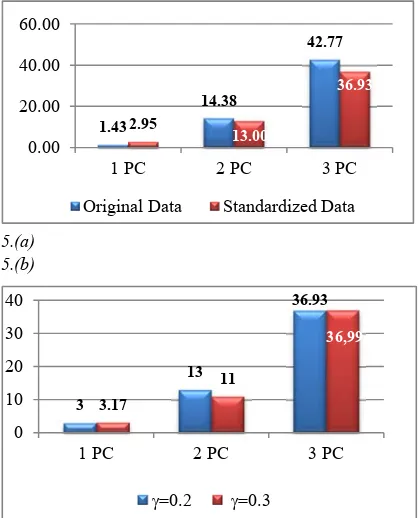
Figure 5 is the result obtained using K-Means clustering algorithm with KPCA transformation. At
= 0.2, the average of SSW (%) for standardized data is smaller than the average of SSW (%) in the original data when using 2 & 3 PCs. The opposite result is the use of 1 PC (Figure 5.a). For standardized data, the average of SSW (%) of clustering using 1 & 3 PCs is not significantly different between = 0.2 and = 0.3. The significant differences occurred in the use of 2 PCs (Figure 5.b), where the average SSW (%) at = 0.2 is greater than the average SSW (%) at = 0.3. The opposite occurs on the average of entropy value (Table 1). In KPCA bandwidth size = 0.3, the clustering results is stable and have very high
internal validation (SSW). These results are better for standardized data than original data on calculations using 2 and 3 PCs, while the opposite is true on the use of 1 PC.
To compare the effect of standardized data on K-Means clustering with KPCA transformation, the entropy value is observeb using 2 PCs with = 0.2.
5.(a) 5.(b)
Figure 5. Percentage SSW of K-Means Clustering Using 1,2 & 3 PCs ( a) = 0.2 On Original and Standardized Data (b) = 0.2 and = 0.3
Entropy value for original data with average ̅ = 0,098 and the variance = 0,024 is higher than entropy value for standardized data with average ̅ = 0.050 and the variance = 0 (Figure 6). This indicates that the clustering of standardized data with = 0.2 has higher accuracy and stable. This means the external validity is optimum.
Figure 6. Entropy of K-Means Clustering on KPCA Bandwidth = 0.2 Using 2 PCs on Original and Standardized Data
0.098
0.050 0.024
0.000 0.000
0.050 0.100 0.150
Original Data Standardized Data Mean Variance
3
13
36.93
3.17
11
36,99
0 10 20 30 40
1 PC 2 PC 3 PC
1.43
14.38
42.77
2.95
13.00
36.93
0.00 20.00 40.00 60.00
1 PC 2 PC 3 PC
5470 The advantage of KPCA bandwidth size
= 0.2 is the clustering results will have a stable (range close to zero) and very high external validation (entropy) even though the calculations are repeated over and over. The entropy value is smaller for the standardized data than the original data on the calculation using 2 PCs.
6. CONCLUSIONS & RECOMMENDATIONS
The analysis of the Iris standardized data that are executed from 30 replications and using 2 PCs show that the size of KPCA bandwidth that ensures the K-Means clustering of non-linearly separable data has high internal and external validation on = 0.2 and = 0.3. The external validity is maximum occurred in bandwidth size
= 0.2 (entropy) and the internal validity is maximum occurred in bandwidth size = 0.3 (percentage of SSW). This results are better than the results of standard K-Means algorithm, either using original or standardized dataset. Standardization of Iris (non-linearly separable dataset), which is transformed into feature space using KPCA, provides clustering results with higher accuracy than using the original data, and that result is very stable.
The empirical results with the optimum bandwidth can be tested on other non-linearly separable datasets or studied mathematically to obtain generalization. Furthermore it can be furtherly investigated to obtain an optimum bandwidth size for high internal and external validity at the same time, then its superiority can be tested on SVC as done by [12].
ACKNOWLEDGMENT
This research was supported by Kementerian Riset, Teknologi dan Pendidikan Tinggi, Republic of Indonesia.
REFERENCES
[1] MacQueen, J. B. 1967. “Some Methods for classification and Analysis of Multivariate Observations”, Proceedings of 5-th Berkeley Symposium on Mathematical Statistics and Probability, Berkeley, University of California Press, Vol. 1, 1967, pp. 281-297. [2] Zhao, Q. “Cluster Validity in Clustering
Methods. Ph.D. Dissertation, University of Eastern Finland”. Publications of the University of Eastern Finland Dissertations in Forestry and Natural Sciences No 77. 2012.
[3] Sakthi, M and A.S. Thanamani. “An Effective Determination of Initial Centroids in K-Means Clustering Using Kernel PCA”. (IJCSIT) International Journal of Computer Science and Information Technologies, Vol. 2 (3), 2011, pp. 955-959.
[4] Souza, C. “Kernel Functions for Machine Learning Applications”. http:// crsouza. blogspot.com/ 2010/03/ kernel-functions- for-machine-learning.html. 17 Mar 2010.
[5] Scholkopf, B., Smola, A., & Muller, K.R. “Kernel principal component analysis. Advances in Kernel Methods”. Support Vector Learning, 10(5), 1999, pp.327–352. [6] Silverman, B.W. “Density Estimation for
statistics and Data Analysis”, Chapman and Hall, London, 1986.
[7] Hoffmann, H. 2007. Kernel PCA for novelty detection. Patt Recogn, 40(3), 863–874. http://doi.org/10.1016/j.patcog.2006.07.009 [8] Tzortzis,G and A. Likas. 2008. “The Global
Kernel K-Means Clustering Algorithm”. International Joint Conference on Neural Networks (IJCNN). 2008, pp. 1978-1985. [9] Chang, Q. ,Chen, Q. and Wang, X. “Scaling
Gaussian RBF Kernel Width To Improve SVMClassification”. ITNLP Lab, School of Computer Science and Technology. Harbin Institut of Technology. Harbin. 150001, China. 2005, pp.19-22.
[10] Lee, S. And K. Daniels. “Gaussian Kernel Width Generator For Support Vector Clustering”. Proceedings. ICBA04. November 4, 2004, pp. 1- 12.
[11] Chen, Q., X. Chen, and Y.Wu. “Optimization Algorithm with Kernel PCA to Support Vector Machines for Time Series Prediction”. Journal of Computers. Volume 5, Number 3, March 2010, pp.380-387.
[12] Kakde, D., Chaudhuri, A., Kong, S., Jahja, M., Jiang, H., & Silva, J. (2016). Peak criterion for choosing Gaussian kernel bandwidth in support vector data description. CoRR,
abs/1602.0, 1–26. Retrieved from http://
arxiv.org/abs/1602.05257. 2016,pp 1–26. [13] Thomas, M., De Brabanter, K., & De Moor, B.
(2014). New Bandwidth Selection Criterion for Kernel PCA: Approach to Dimensionality Reduction and Classification Problems. BMC
Bioinformatics, 15, 137. http://doi.org/
10.1186/ 1471-2105-15-137. 2014.
5471 [15] Mufti, G. B., Bertrand, P., & Moubarki, L. El.
”Determining the number of groups from measures of cluster stability”. Proceedings of International Symposium on Applied Stochastic Models and Data Analysis, 2005, pp. 404-413.
[16] Sripada, S. C and Rao, M.S. 2012. “Comparison Of Purity And Entropy Of K-Means Clustering And Fuzzy C K-Means Clustering”. Indian Journal of Computer Science and Engineering (IJCSE) Vol. 2 No. 3. Jun-Jul 2011, pp 343-346.
5472 APPENDIX
Table 1. Average and Variety of Entropy and SSW on Various KPCA Bandwidth Scales
Bandwidth 0.0001 0.001 0.01 0.1 0.2 0.3 0.4 0.5 0.6 0.7 0.8 0.9
Entropy Mean 0,631 0,668 0,587 0,207 0,050 0,064 0,245 0,174 0,165 0,146 0,103 0,133
Variance 0,019 0,021 0,022 0,000 0,000 0,005 0,045 0,038 0,038 0,044 0,036 0,028
SSW(%) Mean 36,5 37,0 35,1 19,5 13,0 11,0 29,2 26,7 25,6 25,6 23,2 22,7
Variance 3,5 4,85 4,29 0 0 0 413 442 393 337 295 254
Bandwidth 1 2 3 4 5 6 7 8 9 10 100 1000
Entropy Mean 0,174 0,332 0,617 0,693 0,698 0,762 0,785 0,752 0,821 0,819 0,937 0,899
Variance 0,037 0,012 0,016 0,002 0,004 0,000 0,001 0,004 0,000 0,000 0,000 0,026
SSW(%) Mean 27,7 33,0 14,8 20,6 27,4 15,7 14,5 12,5 11,9 11,4 35,3 33,8
Variance 339 221 0 193 363 56 51 0 0 0 443 0
Figure 2. Boxplots of Entropy of Clustering on Various KPCA Bandwidth Scales
Figure 3. Boxplots of Percentage SSW of Clustering on Various KPCA Bandwidth Scales
0.00010.0010.01 0.1 0.2 0.3 0.4 0.5 0.6 0.7 0.8 0.9 1 2 3 4 5 6 7 8 9 10 100 1000 -0.2
0 0.2 0.4 0.6 0.8 1 1.2 1.4
0.00010.0010.01 0.1 0.2 0.3 0.4 0.5 0.6 0.7 0.8 0.9 1 2 3 4 5 6 7 8 9 10 100 1000 -10