Exoplanetary Atmospheric Characterization Using Polarimetry and Other Radiative Transfer Modeling Problems

(1)

Polarimetry and Other Radiative Transfer Modeling

Problems

Thesis by

Pushkar Kopparla

In Partial Fulfillment of the Requirements for the degree of

Doctor of Philosophy

CALIFORNIA INSTITUTE OF TECHNOLOGY Pasadena, California

2018

(2)

Pushkar Kopparla ORCID: 0000-0002-8951-3907

(3)

(4)

ACKNOWLEDGEMENTS

I’d like to thank my teacher, Prof. Yuk Yung, for a great education. I remember my first group meeting, where nearly a dozen different people brought up progress on their work in one or two sentences, and Yuk always knew exactly what issue they were facing. I did not know then that it was possible to have such a command of so many problems at once. Yuk always showed kindness in his own unique way, while running a tight ship. Beyond work, I enjoyed several conversations with him on various topics from politics, history, capitalism, relationships and life in general. I also learned a lot from him about working with people, and how to deal with conflict gracefully.

I’m also grateful to my committee members, Profs. Heather Knutson, Andy Ingersoll and Dave Stevenson. Apart from giving me great advice during my committee meetings, they also worked with me on research projects at different stages in grad school. Some of these projects did not reach a satisfactory conclusion, and that is certainly something I regret and will reflect on. Nonetheless, I was able to work on nearly anything I pleased and learn from these wonderful teachers. Such freedom is a rare and precious thing, and I will always be grateful to the culture of this Division and Caltech in general that enables freestyle research.

Several JPL scientists were vital to much of the work in this thesis, most prominent among them being Vijay Natraj and David Crisp. I’m deeply grateful to Vijay for leading me through the ins and outs of radiative transfer modeling with great patience. And thanks to Dave, who despite his doubly overbooked schedule always made time to attend the Friday meetings to talk about my work. Thanks to Sloane Wiktorowicz for giving me my first telescope observing experience. Also thanks to Mark Swain and members of his group for their valuable advice. Generous funding support from VPL at the University of Washington, courtesy of Prof. Victoria Meadows, and the President’s and Director’s Fund at Caltech were vital to working on exoplanet polarimetry, seen by many as unviable or at least premature. Thanks to Run-Lie Shia and also Shawn Ewald, for their kindness and willingness to help at any time. And of course, thanks to Margaret Carlos for managing all my bureaucratic affairs, to Ulrika Terrones for always being kind and to Irma Black for giving me this great new computer.

(5)

even though everyone is neck deep in their own research and life problems. Though I cannot do full justice in acknowledging everyone’s support, a few special mentions are in order. My thanks to Chris Spalding for coming by to talk in good moods and bad, to Ian Wong, for treating me to many delicious dinners and to Dana Anderson for making sure I could always go to her wonderful birthday parties. Thanks to Mike Wong, for your kindness, good cheer and for the many great experiences we shared together. Also thanks to Peter Gao, for inviting me to his bachelor party that I nearly did not survive, Nancy Thomas and Nathan Stein, for your halloween parties, trivia and other social initiatives. Outside the Division, I’d like to say thanks to Neel Nadkarni, for showing me it was humanly possible to eat that slowly, to Kishore Jaganathan, for not saying out loud his very worst jokes, and to Sumanth Dathathri, for learning to play Dota 2 with me.

(6)

ABSTRACT

This thesis deals with a pair of current problems with the remote sensing of planetary atmospheres. First is the modeling of polarization of scattered light from the atmospheres of exoplanets. With the first such observations becoming possible in the last year, there is a need to understand what these measurements actually mean. To that end, we developed families of radiative transfer models that simulate polarized phase curves for different atmospheric scenarios on hot Jupiters. These models were then used in the interpretation of scattered light from HD 189733b and WASP 12b, two hot Jupiter exoplanets, to determine their albedos and gauge what type of scattering particles might be present in their atmospheres. The last part of this half deals with observing oceans on distant Earth-like exoplanets using polarization from glint off the water surface. Though this measurement is not possible with current telescopes, but it may become accessible in the next decade with a slew of high powered ground and space telescopes in the pipeline.

(7)

PUBLISHED CONTENT AND CONTRIBUTIONS

1. Kopparla, Pushkar, Vijay Natraj, Drew Limpasuvan, Robert Spurr, David Crisp,

Run-Lie Shia, Peter Somkuti, and Yuk L Yung (2017). “PCA-based radiative transfer: Improvements to aerosol scheme, vertical layering and spectral binning”. In: Journal of Quantitative Spectroscopy and Radiative Transfer 198, pp. 104–

111., doi:10.1016/j.jqsrt.2017.05.005

I participated in the conception of the project, set up the model runs, analyzed the results and wrote the manuscript.

2. Kopparla, Pushkar,Vijay Natraj, Robert Spurr, Run-Lie Shia, David Crisp, and

Yuk L Yung (2016). “A fast and accurate PCA based radiative transfer model: Exten-sion to the broadband shortwave region”. In: Journal of Quantitative Spectroscopy

and Radiative Transfer 173, pp. 65–71., doi:10.1016/j.jqsrt.2016.01.014

I participated in the conception of the project, performed the model runs, analyzed the results and wrote the manuscript.

3. Somkuti, Peter, Hartmut Boesch, Vijay Natraj, and Pushkar Kopparla (2017).

“Application of a PCA Based Fast Radiative Transfer Model to XCO2 Retrievals in the Shortwave Infrared”. In: Journal of Geophysical Research: Atmospheres

122.19., doi:10.1002/2017JD027013

I provided information on the use of our PCA-RT technique.

4. Kopparla, Pushkar, Vijay Natraj, Xi Zhang, Mark R Swain, Sloane J Wiktorowicz,

and Yuk L Yung (2016). “A Multiple Scattering Polarized Radiative Transfer Model: Application to HD 189733b”. In: The Astrophysical Journal 817.1, p. 32., doi:10.3847/0004-637X/817/1/32

I participated in the conception of the project, assembled and wrote the code, performed the model runs, analyzed the results and wrote the manuscript.

5. Wiktorowicz, Sloane J, Larissa A Nofi, Daniel Jontof-Hutter, Pushkar Kopparla,

Gregory P Laughlin, Ninos Hermis, Yuk L Yung, and Mark R Swain (2015). “A ground-based Albedo Upper Limit for HD 189733b from Polarimetry”. In: The

Astrophysical Journal 813.1, p. 48., doi:10.1088/0004-637X/813/1/48

(8)

LIST OF ILLUSTRATIONS

Number Page

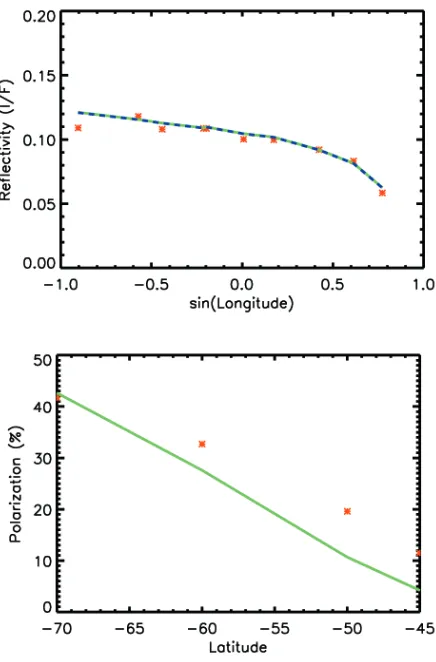
2.1 Top panel shows reflectivities from Zhang et al. (2013) using DIS-ORT(blue dashed line), with this work using VLIDORT (solid green line) and observations from Cassini in the UV1 filter (red points) at S60◦ latitude and a phase angle of 17.5◦. This is the blue curve in the top left panel of Figure 8 in Zhang et al. (2013). Bottom panel shows observed values of polarization in the blue channel from Pio-neer 10 (Smith and Tomasko, 1984, red points) and the corresponding modeled values (this work, solid green line) at a phase angle of 98◦. . 10 2.2 Geometric albedo as a function of single scattering albedo in a

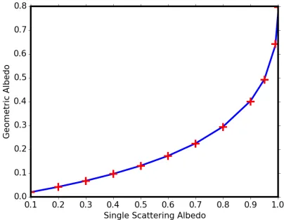
semi-infinite Rayleigh scattering atmosphere from this model (blue curve) and from Madhusudhan and Burrows, 2012 (red pluses). . . 14 2.3 Simple schematic indicating the breakup of the illuminated disk into

smaller regions, each one of which is represented by a stack of plane parallel atmospheric layers. There are N (N typically being 1 or 2) layers which can have either gas alone (Rayleigh scattering) or a mixture of gas and haze particles. This is underlain by a thick, reflective cloud layer at the bottom. Single and multiple scattering (as indicated by the black arrows) are calculated using the radiative tranfer model VLIDORT (Spurr, 2006). . . 17 2.4 Variation in the degree of polarization for reflected light from HD189733b

(11)

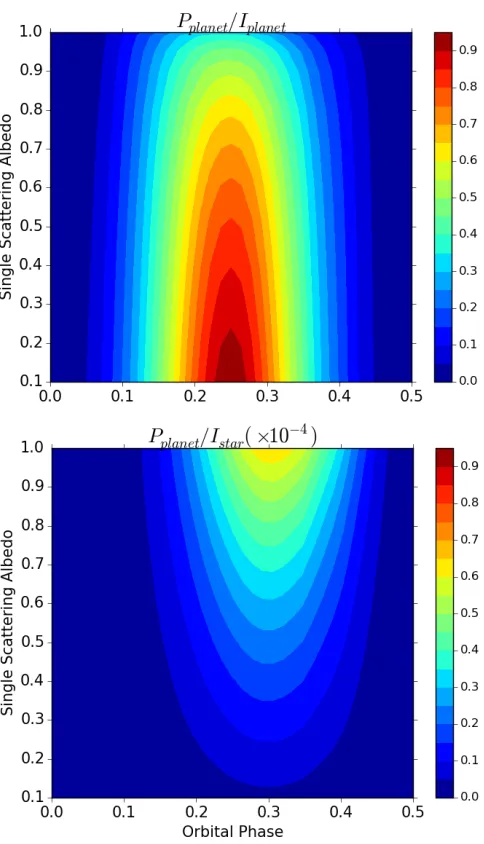
2.5 Variation in the degree of polarization as a function of single scatter-ing albedo and orbital phase for a semi-infinite Rayleigh scatterscatter-ing atmosphere normalized to reflected light from the planet (top) and direct starlight (bottom). For the former, the highest degree of po-larization occurs at low albedo, while for the latter (which is the observable quantity), it occurs at high albedo. . . 20 2.6 Variation in the degree of polarization from reflected light HD189733b

system with a semi-infinite pure gas and hazy atmospheres. The par-ticle properties are listed in Table 2.2. The geometric albedo of the planet is forced to remain close to 0.23. B11 and W09 lines indi-cate the amplitude of observations from Berdyugina et al. (2011) and Wiktorowicz (2009). . . 22 2.7 Variation in reflected intensity and the degree of polarization for

different atmospheric structures of HD 189733b. The intensity curves for a semi-infinite Rayleigh atmosphere (deep gas), thin, clear gas atmosphere (thin gas) and a hazy atmosphere with spherical particles (thin haze) on top of a cloud layer. The haze and cloud properties are mentioned in Table 2.2. . . 23 2.8 Variation in reflected intensity and the degree of polarization as a

planet with an inhomogeneous atmosphere completes one orbit com-pared to a homogeneous, Rayleigh scattering planet. The spheres on top show the planet as seen from Earth at the phases indicated on the abscissa. The dark blue regions are pure Rayleigh scattering, and the greyish regions contain haze. The portion covered by the box indicates the night side of the planet. . . 24 2.9 The top panel shows a cartoon of two orbits of inclination close to 90

(12)

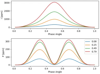
3.1 Scattered light intensity and polarization for Rayleigh scattering at-mospheres on WASP-12b with various geometric albedos. Polariza-tion is expressed as a fracPolariza-tion of direct unscattered starlight in units of parts per million (ppm). . . 36 3.2 Variation of the peak polarization amplitude due to scattering a clear

atmosphere on WASP-12b with geometric albedo. A given value of peak polarization translates directly to a single geometric albedo value of the planet and can be compared to measurements from other techniques such as secondary eclipse (Bell et al., 2017). . . 37 3.3 Polarized light curves for corundum (top) and perovskite (bottom)

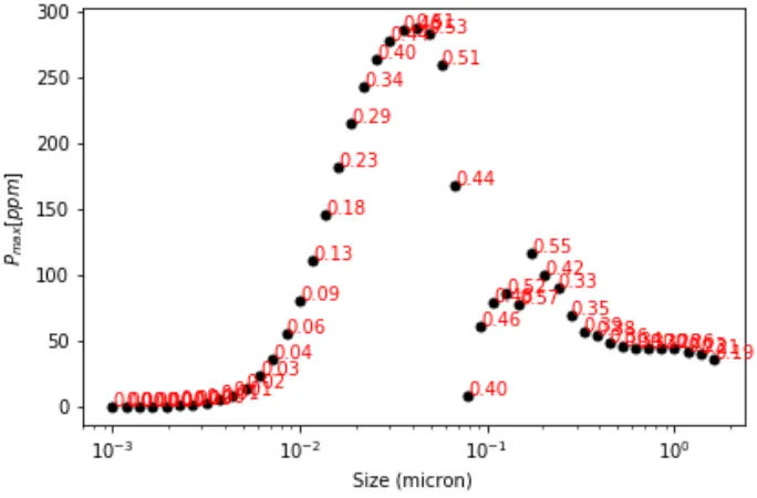
cloud scattering on WASP-12b. Note that peak polarization is a non-monotonic function of particle size. . . 38 3.4 Maximum polarization from the scattering of light by a thick

atmo-spheric cloud on WASP-12b for cloud composed of Al2O3particles of various sizes. The numbers next to the points on the plot indicate geometric albedos for WASP-12b. . . 39 3.5 Same as 3.4, but for a cloud ofCaTiO3particles. . . 40 4.1 Normalized Stokes parameter I and degree of polarization P for a

Cox-Munk glint surface under a very thin 1-D Rayleigh scattering atmosphere (optical depth 0.01) for a variety of values of VZA and AZM. SZA = 60 deg. The wind speed is 1 m/s for the plots in the top row, and 10 m/s for those in the bottom row. . . 46 4.2 A typical total column optical depth spectrum of the Earth’s

(13)

4.3 Reflected starlight intensity and degree of polarization phase curves for TRAPPIST-1e in the thin (left column) and thick atmospheric (right column) limits over an ocean like glinting surface. Legend indicates the optical depth of the atmosphere. The phase angle used here is an atypical convention chosen for consistency with exoplane-tary polarization literature (for e.g., Wiktorowicz et al., 2015). Under this convention, phase angles of 0 and 1 correspond to mid-transit (only nightside is visible) and a phase of 0.5 corresponds to opposi-tion (full dayside is visible). Intensity and polarizaopposi-tion are expressed as fractions of direct, unscattered starlight in units of parts per million [ppm] and parts per billion [ppb]. . . 48 4.4 Same as Fig 4.3, but with scattering by cloud particles of size 2 µm.

Note the appearence of rainbows around phase 0.4 and 0.6 in the thick cloud limit. . . 49 4.5 Phase curves for fully ocean covered (aqua), completely dry planet

and two intermediate cases. The equatorial ocean and global ocean cases have near identical polarization curves since the glint signal comes primarily from near the equator. The intensity curves for the non-dry cases are nearly identical, and different from the dry case, since the dry surfaces are brighter than the ocean at non-glint angles and contribute significantly to disc brightness. . . 51 4.6 Reflected light intensity and polarization expressed as a fraction of

direct starlight for the TRAPPIST-1 system for one period of the outermost planet (∼19 days). Planet e is modeled as an aquaplanet, while the other planets are completely dry. The wet planet signal contributes a much higher fraction of the sum total in polarization (∼ 17%) than in intensity (∼ 1%). . . 53 4.7 Fourier transforms of the combined phase curves (dark black line in

(14)

4.8 Modeled glint star-planet contrast signals (dot-dash grey lines) plot-ted against detection limits of various upcoming large telescopes (WFIRST, LUVOIR and ELT) for systems at a distance of 10 pc. The blue and red lines indicate the distance from the star at which a planet receives an Earthlike (surface water ocean) and Titanlike (sur-face hydrocarbon lakes) solar flux. Present or near future observable Earth like planets (size smaller than 2RE art h) from Kepler detections and candidate objects (downloaded from exoplanets.org (Han et al., 2014) on 6 Oct 2017) and simulated detections from TESS (Sullivan et al., 2015) are overplotted for a sense of the number of detections by surveys that may have an ocean, which can be followed up for glint studies. Planetary periods listed in the TESS simulated dataset are converted to orbital distances by converting the listed stellar radii to stellar masses using the method of Demircan and Kahraman, 1991. . 55 5.1 Top of the Atmosphere (TOA) reflectances from Exact-RT LIDORT

for a single profile showing major absorptions. There are 33 spec-tral fields in all, with 8 in the ultraviolet/visible and the rest in the shortwave infrared (Table 5.1). . . 66 5.2 Residuals (%) of the Exact-RT LIDORT radiances for 2, 4, 8, and 16

streams compared with the 32-streams LIDORT calculations. Optical properties as for Figure 5.1 . . . 67 5.3 Residuals (%) for the PCA (black) and 2S (red) models as compared

to 32 stream LIDORT over the entire shortwave range. The residuals have been Gaussian smoothed to 0.2cm−1. . . 68 5.4 Residuals of the PCA (black) and 2 Stream (red) models as compared

to 32 stream LIDORT with (top) and without (bottom) smoothing for spectral field 9, where the dominant gas absorbers are oxygen and water. . . 69 5.5 The sum total of the runtime of LIDORT and PCA model over all

(15)

5.6 Total column optical depth reconstruction accuracy using 5 EOFs for various settings: (upper left) "standard" PCA on log optical properties on an arbitrarily spaced vertical grid, (upper right) same as standard PCA but with linear optical properties, (lower left) PCA on log opti-cal properties on an equal pressure thickness grid, (lower right) PCA on linear optical properties on an equal pressure thickness grid. Op-tical depths are reconstructed layer by layer and then summed, and compared to the total column optical depth in the original data set. . . 71 5.7 Comparison of PCA RT performance: (top) arbitrarily spaced vertical

grid, (bottom) equal pressure thickness grid. Both grids have 114 layers. RMSE denotes the root mean square error. . . 72 5.8 Differences in PCA RT residuals (bottom) using bin averaging for

aerosol optical properties, and (top) with explicit inclusion of aerosols in the PCA process. Note the almost complete elimination of the slope in the latter scenario. . . 73 5.9 (upper left) TOA radiances, (upper right) residuals using Scheme 1

with 11 bins, (lower left) residuals using Scheme 1 with 21 bins, and (lower right) Scheme 2 with 11 bins, for spectral window 11. The band of absorption lines centered at 0.76µm is the O2 A-band, and that around 0.79µmis due to water vapor absorption. . . 75 5.10 Top of the atmosphere radiances (top left) and residuals using Scheme

2 with 5 bins (top right), 21 bins (bot left) for spectral range 4. Since adding more bins was found to be ineffective with both Schemes 1 (not shown here) and 2, the spectral range was split into two around 0.535µm. Each piece was then treated as a separate spectral range and solved using Scheme 1 binning with 5 bins (bot right). . . 75 5.11 Residuals in spectral window 11 for two diff erent profiles, with

different viewing geometries, aerosol densities and surface types, using Scheme 2 with 11 bins. For a given binning scheme, errors remain fairly constant for different atmospheric profiles taken from the GEOS-CHEM model (Bey et al., 2001). . . 76 5.12 TOA radiances over the entire shortwave range of interest, (top) with

(16)

5.13 Residuals over the entire shortwave range of interest using (top) purely Scheme 2 and (bottom) a combination of Schemes 1 and 2, for a representative atmospheric profile. . . 78 5.14 Mean distribution of residuals over 70 diverse atmospheric profiles

(17)

LIST OF TABLES

Number Page

2.1 Comparisons with Rayleigh Scattering Results of Buenzli and Schmid (2009) . . . 13 2.2 Summary of Parameters Used . . . 17 3.1 Summary of Parameters Used . . . 35 4.1 Scaling factors for brightness to convert above curves to other planets

(18)

C h a p t e r 1

INTRODUCTION

Clouds and hazes are principal constituents of any planetary atmosphere, and their study is vital to understanding of atmospheric radiative properties, dynamics, cli-mates, compositions and chemistry. Clouds and hazes are very well studied on Earth, still somewhat of an enigma on other Solar System planets and pretty much uncharted territory on exoplanets, though this is rapidly changing with the constant influx of observations and the development of increasingly sophisticated atmo-spheric chemistry and dynamical models.

Constraining the composition of hazes observationally on these exoplanets is a hard problem. Since the best observed exoplanets have thus far been hot Jupiters, hazes that can exist in the atmospheres of these very hot planets are typically metal oxides or silicates. There is a lack of easily identifiable spectral features for these species, and uniquely identifying one will require high quality spectra across a broader wavelength range than is currently possible. As a result, we can only infer the presence of clouds or haze due to increased opacity in the atmosphere affecting absorptions by species such as sodium, potassium or water. It is usually possible to narrow the haze candidates based on condensation curves at the expected temperatures, however, a unique determination of haze composition has remained out of reach thus far.

(19)

these effects are regular and the planetary polarization can be retrieved after isolating them. The data is now of sufficient quality to make distinctions between scattering by corundum or perovskite hazes.

The fourth chapter is more of a view towards the future of exoplanet polarimetry. We attempt to answer the question: what will it take to get a direct observation of an ocean on an Earth like exoplanet? Polarimetry is useful here since specular reflection off a water surface is almost 100% linearly polarized. The answer, it seems, depends on a lot of variables: how big the ocean is, how thick the atmosphere and what it’s made of. Though the prospects of such an observation appear bleak at the moment, high powered telescopes that are expected to come online within the next decade might plausibly make it happen.

(20)

C h a p t e r 2

POLARIZATION FROM THE HD 189733 SYSTEM: MODEL

DEVELOPMENT AND INTERPRETATION OF OBSERVATIONS

This chapter is adapted from work previously published as

Kopparla, Pushkar, Vijay Natraj, Xi Zhang, Mark R Swain, Sloane J Wiktorowicz, and Yuk L Yung (2016). “A Multiple Scattering Polarized Radiative Transfer Model: Application to HD 189733b”. In:The Astrophysical Journal817.1, p. 32.

2.1 Abstract

We develop a multiple scattering vector radiative transfer model which produces disk integrated, full phase polarized light curves for reflected light from an exoplanetary atmosphere. We validate our model against results from published analytical and computational models and discuss a small number of cases relevant to the existing and possible near-future observations of the exoplanet HD 189733b. HD 189733b is arguably the most well observed exoplanet to date and the only exoplanet to be observed in polarized light, yet it is debated if the planet’s atmosphere is cloudy or clear. We model reflected light from clear atmospheres with Rayleigh scattering, and cloudy or hazy atmospheres with Mie and fractal aggregate particles. We show that clear and cloudy atmospheres have large differences in polarized light as compared to simple flux measurements, though existing observations are insufficient to make this distinction. Futhermore, we show that atmospheres which are spatially inhomogeneous, such as being partially covered by clouds or hazes, exhibit larger contrasts in polarized light when compared to clear atmospheres. This effect can potentially be used to identify patchy clouds in exoplanets. Given a set of full phase polarimetric measurements, this model can constrain the geometric albedo, properties of scattering particles in the atmosphere and the longitude of the ascending node of the orbit. The model is used to interpret new polarimetric observations of HD 189733b in a companion paper.

2.2 Introduction

(21)

were deduced through polarimetric data from both ground-based observations and from Pioneer data (Hansen and Hovenier, 1974; Kawabata et al., 1980). Similar successful studies exist for Titan (Tomasko and Smith, 1982), Jupiter (Smith and Tomasko, 1984) and the other outer planets (Joos and Schmid, 2007). The idea of using polarimetry to probe exoplanetary atmospheres is thus a natural extension, and was first examined in a theoretical study by Seager, Whitney, and Sasselov (2000). The great advantage of using polarimetry in the study of exoplanets is the increase in contrast between direct starlight and the reflected light from the planetary atmosphere. Integrated over the whole disk, direct starlight from inactive, nearby stars can be assumed to be unpolarized to a high degree1. For instance, the linear polarization integrated over the sun’s disk is∼ 1ppm(parts per million) in visible wavelengths (Kemp et al., 1987), light scattered from a planetary atmosphere may have polarizations of a few tens of percent. Thus, depending on the reflectivity of a planetary atmosphere, the degree of polarization in the star-planet system can be dominated by the reflected light from the planetary atmosphere. In such a case, the combined star planet system should show a periodic modulation in the degree of polarization as the planet moves through different phases of illumination in its orbit.

A prime exoplanet candidate for polarimetric studies is HD 189733b, a hot Jupiter orbiting a K star, with a semimajor axis of 0.031 AU. The system is relatively close by (19.3 parsecs) and thus bright. Berdyugina et al. (2008) reported a detection of polarized light of amplitude 200ppm. Surprisingly, the strength of observed

polarization was about one order of magnitude higher than predicted assuming a semi-infinite Rayleigh scattering atmosphere (which produces the highest degree of polarization for a given planetary radius), leading to some skepticism over the observations (Lucas et al., 2009). Follow up studies since have not reached a consensus on the observed degree of polarization (Wiktorowicz, 2009; Berdyugina et al., 2011). Furthermore, Lucas et al. (2009) observed the polarization of two other exoplanet systems, 55 Cnc andτBoo. In both cases, they found polarization of the order of 1ppm but there was no significant variability associated with the orbital periods of the known exoplanets in these systems. In parallel however, there have been few efforts to model the observable polarization signal using what is known about the atmosphere of HD189733b from photometric measurements, since the early work of Lucas et al., 2009 and Sengupta, 2008. We will briefly examine the

1_{Polarization is introduced in starlight through interactions with interstellar dust clouds and}

(22)

observations, and some of the issues involved in their interpretation, in order to understand what information can be retrieved using a multiple scattering radiative transfer model.

The chapter is structured as follows. The remainder of the introduction is devoted to a review of exoplanetary polarization studies, both theoretical and observational. In Section 2, we outline our model setup and validate our model using observations of Jupiter. In Section 3, we discuss the observable polarization signal for different atmospheric compositions, orbital orientations and spatial inhomogeneities in the atmosphere, followed by a summary in Section 4.

Polarimetry of HD 189733b

Berdyugina et al. (2008)’s study consisted of 93 individual nightly observations taken in the B band (370-550nm) through the KVA 0.6-m telescope and find variable polarization of amplitude 200ppm. The degree of polarization is always measured as a fraction of the direct starlight, and not just the reflected light from the planet. They interpret their observations using a single scattering Rayleigh-Lambertian model, and are able to retrieve values of eccentricity and orbital inclination that agree quite well with other studies. To explain the large degree of polarization, they are forced to use a large planetary radius, 1.5±0.2 RJ where the standard value is 1.154±0.017RJ(Pont et al., 2007). They comment that this large radius might be indicative of an extended, evaporating halo around the planet. It is uncertain if such a halo would be reflective enough to be responsible for a significant fraction of the reflected intensity.

Wiktorowicz (2009) observed the same planet in the wavelength range 400-675 nm from the Palomar 5-m telescope. He found polarization of the order of 10ppm, but there was no significant relationship with the period of the exoplanet. However, this study has only one observation near elongation (phase angle 90◦) where polarization is expected to peak and most observations are at phases where polarization is expected to be small, as has been pointed out by later papers (Berdyugina et al., 2011). This study also derives an upper limit to the polarimetric modulation of the exoplanet as 79ppmand the polarimetric variability of starspots to 21ppm.

(23)

value of the amplitude of polarization from 200ppmdown to∼ 100ppm. Because of the visual similarities to Neptune in the geometric albedo profile, they suggest that the atmosphere might have a similar structure, with a high altitude haze layer above a semi-infinite cloud deck. Another proposed structure is the presence of a dust condensate layer beneath a thin gas layer.

Photometric Observations

Temperatures in the atmosphere of HD 189733bare thought to vary between 1000-1500 K depending on altitude and longitude (Knutson et al., 2009; Knutson et al., 2012; Huitson et al., 2012). Its atmosphere is fairly well studied and is known to contain water (Tinetti et al., 2007), carbon monoxide (Kok et al., 2013), carbon dioxide and methane (Swain, Vasisht, and Tinetti, 2008; Swain et al., 2009) in trace amounts. The bulk composition is usually modeled to be mostly hydrogen and helium (Huitson et al., 2012; Danielski et al., 2014). From theoretical models, it is also expected that such an atmosphere would contain traces of metals like sodium, potassium and magnesium (Fortney et al., 2010). Weak detections of these metals from visible (Redfield et al., 2008) and infrared transmission spectra as well as strong slope from the UV to the near infrared, lead to the inference that a high level, Rayleigh haze that spans several scale heights over an opaque cloud deck may be present (Sing et al., 2009; Désert et al., 2011; Sing et al., 2011; Pont et al., 2013).

However, a recent pair of studies (Crouzet et al., 2014; McCullough et al., 2014) have put forth an alternative interpretation of the transit and secondary eclipse data. They argue that the slope previously attributed to a Rayleigh scattering haze could instead be caused by unocculted star spots in the field of view. This interpretation favors a clear, cloudless atmosphere for HD 189733b, though it does not rule out a hazy atmosphere.

The geometric albedo of HD 189733b was measured by Evans et al. (2013) using the HST to measure the brightness of the disk at secondary eclipse, and they find values of 0.40±0.12 in the range 290-450 nm and an upper limit of 0.12 between 450-570 nm. This data provides an independent check for the albedos retrieved by Berdyugina et al. (2011). The values of Berdyugina et al. (2011) are systematically higher than those obtained by Evans et al. (2013).

Theoretical Polarization Studies

(24)

ra-diative transfer (RT) model for a Rayleigh scattering atmosphere. They concluded that the maximum degree of polarization (1 −5x10−5) was in most cases below detection limits at the time. They also examined the effects of scattering particles and cloud layers, in all cases deviation from a purely scattering gaseous atmosphere reduced the degree of polarization. Following this, there were a series of papers e.g., Stam, Hovenier, and Waters (2004) and Stam et al. (2006) using an adding doubling RT model. Their results were similar to that of the previous work, but the great advantage of their model is the generation of a "planetary scattering matrix". With this matrix, a single calculation can replicate multiple scattering radiative transfer through a planetary atmosphere of arbitrary thickness and composition (only for top of the atmosphere fluxes). Buenzli and Schmid (2009) explored the dependence of observable polarization signals on single scattering albedo, optical depth of the scattering layer, and albedo of an underlying Lambert surface for purely Rayleigh scattering atmospheres using a Monte Carlo model. Madhusudhan and Burrows (2012) used an analytic model on a Rayleigh scattering atmosphere to map out polarization signals for various scenarios.

(25)

2.3 The Atmospheric Structure of HD 189733b and Radiative Transfer Model Setup

Our approach to building an exoplanetary atmospheric polarization model is to start with a well understood planetary atmospheric model, continually modify into an atmospheric structure relevant to HD 189733b and validate it at each step. We begin with a model of Jupiter’s stratosphere based on retrievals of Cassini data (Zhang et al., 2013), henceforth Z13. This model is attractive as a baseline since the atmosphere has realistic clouds and two different types of haze particles: spherical and fractal aggregates. While current polarimetric observations may not have sufficient data to distinguish between these two types of haze particles, we are optimistic about the future. Z13 model the atmosphere of Jupiter using a 12-layer plane parallel atmosphere with scattering and absorption at each layer, underlain by a reflective semi-infinite cloud layer. This model currently works only with the photometric intensity,I, while we require at least three of the Stokes parameters,I, the intensity, and Q and U, the linear polarization parameters.The degree of polarization, P is defined as

P = p

Q2+_U2 Istar+Iplanet

∼

p

Q2+_U2

Istar (2.1)

(26)

usual Lambertian surface assumption. The VLIDORT model is also fully linearized: simultaneously with the polarized radiance field, it will deliver analytic Jacobians with respect to any atmospheric and/or surface properties.

VLIDORT has been validated against Rayleigh (Coulson, Dave, and Sckera, 1960) and aerosol benchmark results (Garcia and Siewert, 1989; Siewert, 2000). Details of the validation can be obtained from Spurr (2006). VLIDORT has also been validated in the thermal infrared (with no solar sources) and mid infrared (with both solar and thermal emission sources) spectral regions by comparisons with the National Center for Atmospheric Research GENLN Spectral Mapper model, which in turn is based on the GENLN line-by-line RT algorithm (Edwards, 1992). VLIDORT has been previously used in remote sensing applications for Earth (Cuesta et al., 2013; Xi et al., 2015).

(27)

[image:27.612.198.416.103.434.2]

are discussed in the following section on disk integration.

Figure 2.1: Top panel shows reflectivities from Zhang et al. (2013) using DIS-ORT(blue dashed line), with this work using VLIDORT (solid green line) and observations from Cassini in the UV1 filter (red points) at S60◦latitude and a phase angle of 17.5◦. This is the blue curve in the top left panel of Figure 8 in Zhang et al. (2013). Bottom panel shows observed values of polarization in the blue channel from Pioneer 10 (Smith and Tomasko, 1984, red points) and the corresponding modeled values (this work, solid green line) at a phase angle of 98◦.

Disk Integration

(28)

UandV. I=           I Q U V           (2.2)

The integral of interest, which gives the integrated Stokes parameters of the planet over the illuminated fraction of the disk at a phase angleα, is

j(α)=

∫ π

0

sin2ηdη ∫ π

α−π/₂

I(η, ζ)cosζdζ _(2.3)

whereI(η, ζ)is the outgoing Stokes vector from the point defined by the colatitude ηand longitudeζ in the direction of the observer. The intensity within the integral

is not analytical and must be obtained from multiple scattering calculations from VLIDORT. It is therefore preferable to have the integral expressed as a summation over some finite number of points. Using the transformation

ξ =

2 cosα+1

ν+

cosα

−₁

cosα+1

, ψ= cosη (2.4)

whereν = sinη, the limits of the integrals are changed to -1 to +1. Note that these equations are valid for positive phase angles, α. For negative phase angles, the extent of the illuminated disk is expressed as

j(α)=

∫ π

0

sin2η dη ∫ π−α

−π/₂

I(η, ζ)cosζdζ _(2.5)

The corresponding variable substitution is now

ξ =

2 cosα+1

ν−

cosα₋ 1 cosα+1

, ψ= cosη (2.6)

These integrals can now be expressed as the summations

j(α)= (cosα+1)

2 n Õ i=1 n Õ j=1

wiujI(ψi, ξj) (2.7)

where eachwiandujrepresents the quadrature weights for the quadrature divisions ψi andξj. For a given number of summation terms, n, the quadrature weights and

(29)

the outgoing intensity. The inputs to VLIDORT are the solar zenith angle (θo), indicating the direction of the incoming flux from the star measured with respect to the local normal to the surface, viewing zenith angle (θo), which is the direction of outgoing radiance to the observer, and the relative azimuthal angle (∆φ) between these two directions. These angles are given by

cosθo=sinηcos(η−α) (2.8)

cosθ =sinηcos(η) (2.9)

tan∆φ= sinαcosη

cosθcosθo−cosα (2.10)

We verify that our numerical implementation is correct by reproducing Table 3 of Horak (1950) for surface reflection from a Lambertian surface.The effects using different numbers of quadrature points, computational streams in the RT model and the resolution of the orbit are discussed in the appendix. In brief, pure Rayleigh scattering atmospheres are insensitive to resolution effects and use 8-stream, 64-point quadrature. Mie scattering atmospheres require at least 16-stream RT to produce rainbows and use 32-stream and 256-point quadrature for the cases discussed. For inhomogeneous hazy atmospheres with sharp discontinuities in the scattering properties across the disk, 32-stream, 1024-point quadrature was used to produce smooth curves in reflected intensity. Model runtime scales linearly with number of phases modeled per orbit, as the square of the linear spatial resolution of the disk and the cube of the number of RT streams.

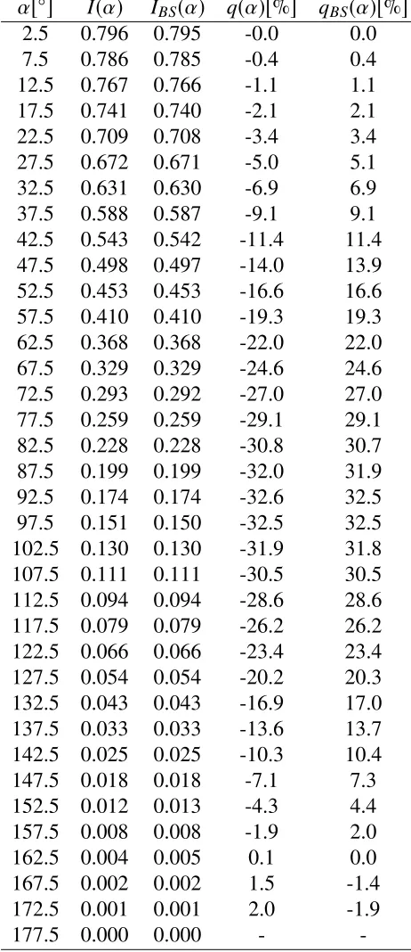
To further validate our disk integration scheme implementation, we reproduce the disk integrated reflectivity and degree of polarization calculations from Buenzli and Schmid (2009) for Rayleigh scattering atmosphere of optical depth 30 and single scattering albedo 0.999999 over a Lambertian surface of albedo 1. Our results agree well with published values, as shown in Table 2.1. The error in the degree of polarization is given as 0.1% in Buenzli and Schmid, 2009. The columns are the scattering phase angle (α), reflectivity (I, this work, IBSfrom (Buenzli and Schmid, 2009)) and the degree of polarization expressed as a percentage of reflected light (q andqBS respectively). In this work, we use the definitions of the Stokes parameters

as given by Hovenier, Mee, and Domke, 2014, which are the same as those used in Chandrasekhar, 1960. Buenzli and Schmid, 2009 use the definition from Coulson, Dave, and Sckera, 1960, which only differs in the sign ofQ.

(30)

[image:30.612.188.419.114.648.2]

Table 2.1: Comparisons with Rayleigh Scattering Results of Buenzli and Schmid (2009)

α[◦] I(α) IBS(α) q(α)[%] qBS(α)[%]

2.5 0.796 0.795 -0.0 0.0

7.5 0.786 0.785 -0.4 0.4

12.5 0.767 0.766 -1.1 1.1

17.5 0.741 0.740 -2.1 2.1

22.5 0.709 0.708 -3.4 3.4

27.5 0.672 0.671 -5.0 5.1

32.5 0.631 0.630 -6.9 6.9

37.5 0.588 0.587 -9.1 9.1

42.5 0.543 0.542 -11.4 11.4 47.5 0.498 0.497 -14.0 13.9 52.5 0.453 0.453 -16.6 16.6 57.5 0.410 0.410 -19.3 19.3 62.5 0.368 0.368 -22.0 22.0 67.5 0.329 0.329 -24.6 24.6 72.5 0.293 0.292 -27.0 27.0 77.5 0.259 0.259 -29.1 29.1 82.5 0.228 0.228 -30.8 30.7 87.5 0.199 0.199 -32.0 31.9 92.5 0.174 0.174 -32.6 32.5 97.5 0.151 0.150 -32.5 32.5 102.5 0.130 0.130 -31.9 31.8 107.5 0.111 0.111 -30.5 30.5 112.5 0.094 0.094 -28.6 28.6 117.5 0.079 0.079 -26.2 26.2 122.5 0.066 0.066 -23.4 23.4 127.5 0.054 0.054 -20.2 20.3 132.5 0.043 0.043 -16.9 17.0 137.5 0.033 0.033 -13.6 13.7 142.5 0.025 0.025 -10.3 10.4 147.5 0.018 0.018 -7.1 7.3 152.5 0.012 0.013 -4.3 4.4 157.5 0.008 0.008 -1.9 2.0

162.5 0.004 0.005 0.1 0.0

167.5 0.002 0.002 1.5 -1.4

172.5 0.001 0.001 2.0 -1.9

177.5 0.000 0.000 -

-(Signs are opposite due to the use of different conventions. See text for details)

(31)

[image:31.612.199.401.218.375.2]

expres-sion from Madhusudhan and Burrows (2012), shown in Figure 2.2. We get good agreement except close to single scattering albedo ∼ 1, where the analytic fitting expression is not good as reported by Madhusudhan and Burrows, 2012. However, our model value of 0.7976 is close to the published numerically computed values of 0.7977 (Madhusudhan and Burrows, 2012) and 0.7975 (Prather, 1974). VLIDORT cannot handle a single scattering albedo of exactly 1, and therefore we use the value 0.999999.

Figure 2.2: Geometric albedo as a function of single scattering albedo in a semi-infinite Rayleigh scattering atmosphere from this model (blue curve) and from Madhusudhan and Burrows, 2012 (red pluses).

Geometric Considerations

For a circular orbit, we have the scattering angle for a given orbital position (Mad-husudhan and Burrows, 2012)

cosα=sinφsini (2.11)

(32)

parametersI andV remain unchanged since they deal with the total intensity and the handedness and magnitude of circular polarization. Thus the first rotation is of the form (Madhusudhan and Burrows, 2012)

          I0 Q0 U0 V0           =          

1 0 0 0

0 cos 2γ1 sin 2γ1 0 0 −sin 2γ1 cos 2γ1 0

0 0 0 1

                    I Q U V           (2.12)

cosγ1=

sinη sinζ

sinθ (2.13)

θis the angle with the vertical at the point of scattering made by the outgoing beam

of radiation to Earth. The angle of the second rotation is a function of the planet’s position in the orbit and is given by (Schmid, 1992)

γ₂=tan−1

tanφ cosi

+90◦+ωp (2.14)

whereiis the inclination of the orbit andωpis the longitude of the ascending node. Note that the orbit is assumed to be nearly circular, which is valid for HD 189733b. The rotation itself is of the form

Q00= Q0cos 2γ2 (2.15)

U00 =Q0sin 2γ2 (2.16)

I and V are unaffected as before. Note that U0 plays no role in the second

rota-tion since its value drops to zero during the first rotarota-tion and summarota-tion over the illuminated disk for a planet that is symmetric about its equator. This set of trans-formations yield the full orbit polarized phase curve[I(φ),Q00(φ),U00(φ),V(φ)]for the planet. Our simple model does not account for transit, secondary eclipse or limb effects in the star and the planet, non-spherical planets, thermal emission from the planet and other higher order effects. Those will be considered in future efforts.

Atmospheric Structure of HD 189733b

(33)

0.99. Gas is also present in this layer; however, the large optical depth of the cloud makes scattering by gas inconsequential within this layer. A simple schematic of this plane parallel atmosphere is provided in Figure 2.3. Since we do not require this level of vertical resolution with current observations, we will reduce the number of gas layers, N to 1 or 2 depending on the case of interest. Should observations of sufficient quality become available, it is easy to add on more layers. The cloud layer is underlain by a Lambertian surface of albedo zero to provide a boundary condition. However, the cloud layer is thick enough (τcloud = 50) that changes to the albedo of this surface has no observable effect. The atmospheric composition of HD 189733b consists primarily of hydrogen and helium, with traces of methane, carbon dioxide and water. Since none of these gases have absorption lines or bands at 0.44µm, their contribution is primarily Rayleigh scattering. We take the typical depolarization ratio of 0.02 for hydrogen as representative of the atmosphere follow-ing Stam, Hovenier, and Waters (2004). The scatterfollow-ing properties of the underlyfollow-ing cloud layer is described by a double Henyey-Greenstein (DHG) function, Equation 2 of Z13. The DHG function is fully depolarizing. For the sake of simplicity and due to the lack of better alternatives, we use the following values from Table 4 of Z13 for the parameters for the double Henyey-Greenstein scattering function, f1 = 0.8303,

g₁ =0.8311 andg2= −0.3657. A summary of relevant atmospheric parameters is provided in Table 2.2. The total column optical depth of the gaseous atmosphere (excluding the bottom cloud layer) is treated as a free parameter. However, we find that with total column optical depths of order one, a doubling or halving of the optical depth only results in changes of order 5-10% in the intensity and degree of polarization for a pure Rayleigh scattering atmosphere.

(34)

Figure 2.3: Simple schematic indicating the breakup of the illuminated disk into smaller regions, each one of which is represented by a stack of plane parallel atmospheric layers. There are N (N typically being 1 or 2) layers which can have either gas alone (Rayleigh scattering) or a mixture of gas and haze particles. This is underlain by a thick, reflective cloud layer at the bottom. Single and multiple scattering (as indicated by the black arrows) are calculated using the radiative tranfer model VLIDORT (Spurr, 2006).

Table 2.2: Summary of Parameters Used

Function Parameter Value

Wavelength 0.44 µm

Cloud Ph. Fn. (DHG) f1 0.8303

g1 0.8311

g2 -0.3657

Haze Particles Refractive Index 1.68+10−4i Radius (spherical) 1µm Monomer radius (fractal) 10nm

Monomers/particle 1000

for all gases, haze and cloud particles. The planetary and orbital parameters for HD 189733b are taken as follows. The radius of the planet is 1.138Rj, semi-major axis is 0.03 AU and the eccentricity of the orbit is taken to be nearly zero (actual value is 0.0041) (Torres, Winn, and Holman, 2008). The inclination of the orbit can be either 86◦ (Triaud et al., 2010; Berdyugina et al., 2008) or 94◦(Berdyugina et al., 2011)(we use 94◦) and the longitude of the ascending node is 16◦(Berdyugina et al., 2008).

2.4 Results and Discussion

(35)

po-larization over the northen and southern hemispheres will likely have comparable absolute values but opposite signs. The result is that integrated over the disk, the circular polarization values are very small. The degree of circular polarization is at least 4-5 orders of magnitude smaller than the linear polarization, and cannot be measured with current technology for exoplanets. Thus, the reflected light from the atmosphere of an exoplanet is described fully by I, Q and U. The total degree of polarization of reflected light is wholly determined by the nature of scattering in the planetary atmosphere, while the viewing geometries determine the distribution of polarization between the parameters QandU. The broad atmospheric structure of HD 189733b is still a matter of active debate. Depending on the interpretation of transit spectra, cloudy or clear atmospheric scenarios cannot be ruled out (Crouzet et al., 2014). Thus, we will examine a few simple structures and their associated polarization signatures here.

Semi-infinite Rayleigh Scattering Atmospheres

(36)

For a purely Rayleigh scattering atmosphere, the degree of polarization depends only on the single scattering albedo. The single scattering albedo accounts for the presence of absorbing gases in that layer. Since each photon is scattered around till it is either absorbed or leaves the atmosphere, layers with high albedo have multiple scattering that randomizes the plane of polarization and reduces the observed degree of polarization at the top of the atmosphere. One might be tempted to infer, therefore, that low albedos are preferable to reduce multiple scattering and have larger polarization signals. However, as the albedo of the atmosphere is lowered, the planet becomes dimmer with respect to the star. Consequently, the maximum degree of polarization in the star-planet flux becomes lesser. These two competing albedo effects give rise to different behaviors depending on whether the polarization is normalized to the intensity of the star or the reflected intensity of the planet as seen in Figure 2.5.

Figure 2.4: Variation in the degree of polarization for reflected light from HD189733b with changes in geometric albedo for a semi-infinite, purely Rayleigh scattering atmosphere. I and P are normalized to direct starlight. The B11 and W09 lines indicate the amplitude of observations from Berdyugina et al. (2011) and the upper limit for non-detection from Wiktorowicz (2009). Orbital phase 0 is mid-transit and 0.5 is mid-eclipse.

(37)

[image:37.612.184.426.69.491.2]

Figure 2.5: Variation in the degree of polarization as a function of single scattering albedo and orbital phase for a semi-infinite Rayleigh scattering atmosphere normal-ized to reflected light from the planet (top) and direct starlight (bottom). For the former, the highest degree of polarization occurs at low albedo, while for the latter (which is the observable quantity), it occurs at high albedo.

Semi-infinite Hazy Atmospheres

Based on the interpretation of Pont et al. (2013) and others, the atmosphere of HD 189733b consists of a well-mixed Rayleigh scattering haze over several scale heights. To model this, we introduce two types of scattering particles into the atmosphere: spherical particles of size 1µm and fractal particles of effective size

(38)

in shape to fractal particles used in Z13, but their refractive index is that of silicates, 1.68+10−4i. As in Section 3.2, a single gas+haze layer with an optical depth of 1000 makes up the atmosphere, with an underlying cloud layer. These particles are added such that they contribute to 50% of the optical depth at each atmospheric layer, while the geometric albedo is held constant close to 0.23. This is achieved by setting the single scattering albedo to 0.71 in the Rayleigh case, 0.54 in the Mie case and 0.84 in the fractal case. The resulting curves are shown in Figure 2.6.2 The highest polarization is always produced by a non-absorbing, purely Rayleigh scattering atmosphere. The introduction of any particle that deviates from this regime reduces the polarization. Polarization is non-zero at orbital phase 0.5 since the planet is in an orbit whose inclination is not 90◦. Therefore, at this orbital phase the phase angle is∼ 4◦, while polarization is zero for a phase angle of 0◦.

A simple reason to explain this effect is that moving from the Rayleigh to Mie regime reduces reflection at quadrature angles and increases preferential forward scattering. Since the polarization peak occurs near quadrature, and there is lower reflection at this point, the total degree of polarization invariably decreases. The fractal particles are characterized by their Mie particle-like intensity curve, which comes from their large effective radius and Rayleigh-like polarization curve, which is due to the small size of individual monomers that make up the aggregate. The Mie-particle haze can be distinguished by a rainbow close to secondary eclipse. Thus, for a given albedo, using a combination of intensity and polarization measurements, it should be possible to determine whether a haze is present, and what type of particles might be present in it. Recent work has begun to place constraints on scattering particle properties (Muñoz and Isaak, 2015). Increasing effective haze particle size decreases the degree of polarization observed. However, it will be tricky to characterize the size of haze particles from the degree of polarization alone without extremely high resolution polarimetric observations (∆P∼few ppm).

Thin Atmospheres Above Cloud Decks

Berdyugina et al., 2011 proposed an atmospheric structure with a thin gas or haze layer on top of a semi-infinite cloud or condensate deck. Since the nature of the cloud or haze layer remains fairly unconstrained in this picture, we create a structure with two layers. In the first case, the top layer is pure gas with an optical depth of 1.0,

2

(39)

Figure 2.6: Variation in the degree of polarization from reflected light HD189733b system with a semi-infinite pure gas and hazy atmospheres. The particle properties are listed in Table 2.2. The geometric albedo of the planet is forced to remain close to 0.23. B11 and W09 lines indicate the amplitude of observations from Berdyugina et al. (2011) and Wiktorowicz (2009).

(40)

Figure 2.7: Variation in reflected intensity and the degree of polarization for different atmospheric structures of HD 189733b. The intensity curves for a semi-infinite Rayleigh atmosphere (deep gas), thin, clear gas atmosphere (thin gas) and a hazy atmosphere with spherical particles (thin haze) on top of a cloud layer. The haze and cloud properties are mentioned in Table 2.2.

Inhomogeneous Atmospheres

Thus far we have considered homogeneous atmospheres, in both the vertical and horizontal directions, which are idealized cases. We treat one case of horizontal inhomogeneity, where one hemisphere is covered by a haze and the other hemisphere is clear. Such scenarios are of particular interest, since haze and cloud formation process often produce patchy, inhomogeneous regions as seen in the Solar System planets and brown dwarfs. A recent study of the exoplanet Kepler 7b indicates the presence of spatial inhomogeneity where one hemisphere of the planet is more reflective than the other (Demory et al., 2013; Hu et al., 2015), possibly indicating that one hemisphere is covered by patchy clouds while the other is clear.

(41)

at quadrature as compared to the reflected intensity.

[image:41.612.187.423.335.565.2]

Numerically, we create two different atmospheric structures. All longitudes west of the substellar point (which lies at the longitude equal to the scattering angle,α) correspond to the clear structure, eastward are hazy. Thus far, we have usedα as defined by Equation 4, which only yields non-negative values. We can get away with only positive α for a homogeneous planet because of longitudinal symmetry. For an inhomogeneous planet, we must have negativeαvalues betweenφ = [π,2π]to ensure that the correct scattering angles are used. Inhomogeneous atmospheres have been modeled by Karalidi and Stam, 2012; Karalidi, Stam, and Guirado, 2013, by calculating the brightness of homogeneous planets and creating an inhomogeneous planet from their area-weighted averages. One advantage of this method is that we do not need to repeat calculations for different homogeneous planets before arriving at the inhomogeneous case.

(42)

Dependence on Orbital Parameters

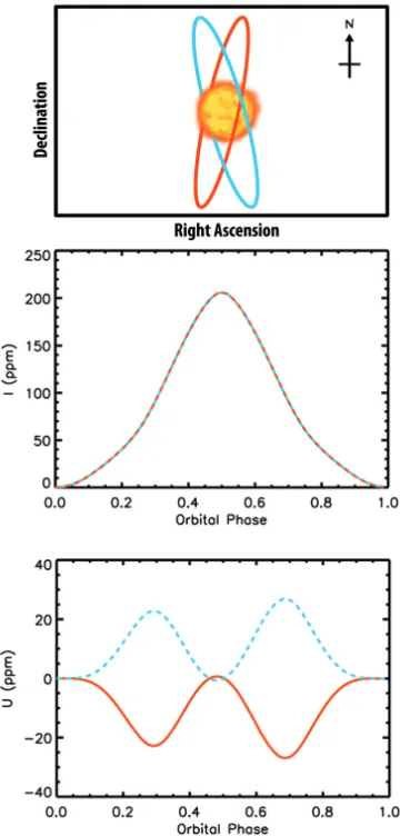
The range of observed phase angles for one orbit of the exoplanet around the star is set entirely by its inclination. For instance, an inclination of 0◦, allows only a constant phase angle of 90◦, while an inclination of 90◦ allows the full range from 0−180◦. Intermediate values of inclination allow smaller ranges of phase angles to be observed. Since the inclination can usually be inferred from the transit light curve, we do not consider it a free parameter. However, the longitude of the ascending node cannot always be pin pointed from photometric light curves alone. Figure 2.9 shows an example of two possible transiting orbit candidates for an exoplanet which have the same inclination, but longitudes of the ascending node are of opposite sign albeit same magnitude. The first panel shows the photometric light curve, which is identical for both orbits and cannot be used to distinguish them, while the polarimetric curve,U, clearly shows a change in sign.

2.5 Conclusions

In this paper, we describe a multiple scattering radiative transfer model capable of generating polarized phase curves for reflected light from a range of atmospheric structures. In general, we find that our multiple scattering model cannot produce polarization high enough to match the observations of Berdyugina et al., 2011, agreeing with the findings of Lucas et al., 2009. We also find that clear and hazy atmospheres have observable differences in polarized light. In combination with full orbit reflected intensity phase curves, it might be possible to even distinguish if the haze particles are spheres or aggregates. Furthermore, we also find that spherical haze particles with the refractive of silicate have a rainbow, and corresponding peak in polarization, close to secondary eclipse. In addition, we examine cases where a thin atmosphere is underlain by a semi-infinite cloud layer, and find that they are distinguishable from semi-infinite clear gas atmospheres. The semi-infinite Rayleigh scattering cases were used to put an upper limit on the albedo of HD 189733b in the visible in a companion paper (Wiktorowicz et al., 2015)

(43)

[image:43.612.218.398.83.459.2]

Figure 2.9: The top panel shows a cartoon of two orbits of inclination close to 90 degrees and longitude of the ascending node 16 degrees (red, solid line) and -16 degrees (blue, dashed line) for the HD189733b system as seen from Earth. (Figure is approximate, not to scale, angles are not accurately depicted). The arrow indicates the sense of motion of the planet in the orbit and upwards is North in the sky plane of the Earth. These orbits are indistinguishable from photometry alone, but can be separated using polarimetry. The sign of Stokes parameter U changes, while intensity is invariant for this pair of orbits.

(44)

We show in this paper that contrasts between clear skies and fully or patchy clouds are significant in polarized light even when the reflected light intensities cannot be differentiated. The locations of hazes and clouds, combined with temperature profiles, can be used to infer the composition of the condensates based on their condensation temperatures. While intensity phase curves may yield information about the size of the scattering particle, polarized curves also give information about the refractive index depending on the position of the rainbow, allowing for additional constraints on chemical composition. The size of cloud particles is indicative of the strength of the updrafts necessary to buoy them, among other factors (see Reutter et al., 2009 for example,) and can provide constraints on the dynamics of exoplanetary atmospheres. The closeness of hot Jupiters to their stars, and the resulting interactions with stellar magnetospheres, can influence the chemistry of the atmosphere. In the solar system, it is thought that the magnetosphere of Jupiter plays a key role in the creation of fractal aggregate hazes near the polar regions (Wong, Yung, and Friedson, 2003).

Better constraints on the scattering properties of atmospheric particles and con-densates will allow for the understanding of their formation mechanisms, which are linked to the circulation of the atmosphere itself. Though our model uses overly simplified atmospheric structures in its present form, future work will in-clude spatial variations in atmospheric composition and structure in a more rigorous fashion. One possible extension might be to generate clouds and hazes through a 3D general circulation model and perform vector radiative transfer on the resulting atmospheric structures. As polarimetric observations converge on acceptable val-ues for HD189733b, and new observations become available for other exoplanets, our model can be used in a retrieval framework to constrain atmospheric scattering properties and orbital elements.

2.6 Acknowledgements

(45)

References

Bailey, Jeremy (2007). “Rainbows, polarization, and the search for habitable plan-ets”. In:Astrobiology7.2, pp. 320–332.

Berdyugina, SV, AV Berdyugin, DM Fluri, and V Piirola (2011). “Polarized re-flected light from the exoplanet HD189733b: first multicolor observations and confirmation of detection”. In:The Astrophysical Journal Letters728.1, p. L6.

Berdyugina, Svetlana V, Andrei V Berdyugin, Dominique M Fluri, and Vilppu Piirola (2008). “First detection of polarized scattered light from an exoplanetary atmosphere”. In:The Astrophysical Journal Letters673.1, p. L83.

Buenzli, Esther and Hans Martin Schmid (2009). “A grid of polarization models for Rayleigh scattering planetary atmospheres”. In: Astronomy & Astrophysics 504.1, pp. 259–276.

Chandrasekhar, Subrahmanyan (1960).Radiative transfer. Courier Dover Publica-tions.

Coulson, Kinsell L, Jitendra V Dave, and Z Sckera (1960). “Tables related to radia-tion emerging from a planetary atmosphere with Rayleigh scattering”. In:

Crouzet, Nicolas, Peter R McCullough, Drake Deming, and Nikku Madhusudhan (2014). “Water Vapor in the Spectrum of the Extrasolar Planet HD 189733b. II. The Eclipse”. In:The Astrophysical Journal795.2, p. 166.

Cuesta, Juan et al. (2013). “Satellite observation of lowermost tropospheric ozone by multispectral synergism of IASI thermal infrared and GOME-2 ultraviolet mea-surements over Europe”. In:Atmospheric Chemistry and Physics13.19, pp. 9675– 9693.

Danielski, C, P Deroo, IP Waldmann, MDJ Hollis, G Tinetti, and MR Swain (2014). “0.94-2.42 µm Ground-based Transmission Spectra of the Hot Jupiter HD-189733b”. In:The Astrophysical Journal785.1, p. 35.

Davis, Leverett and Jesse L. Greenstein (May 1949). “The Polarization of Starlight by Interstellar Dust Particles in a Galactic Magnetic Field”. In:Phys. Rev.75 (10), pp. 1605–1605. doi:10.1103/PhysRev.75.1605. url:http://link.aps.

org/doi/10.1103/PhysRev.75.1605_.

De Rooij, WA and CCAH Van der Stap (1984). “Expansion of Mie scattering matrices in generalized spherical functions”. In: Astronomy and Astrophysics 131, pp. 237–248.

Demory, Brice-Olivier et al. (2013). “Inference of inhomogeneous clouds in an exoplanet atmosphere”. In:The Astrophysical Journal Letters776.2, p. L25.

Désert, J-M, D Sing, A Vidal-Madjar, G Hébrard, D Ehrenreich, A Lecavelier Des Etangs, V Parmentier, R Ferlet, and GW Henry (2011). “Transit spectrophotom-etry of the exoplanet HD 189733b-II. New Spitzer observations at 3.6 µm”. In:

(46)

Edwards, DP (1992). “GENLN2: A general line-by-line atmospheric transmit-tance and radiance model. Version 3.0: Description and users guide”. In: Rep.

NCAR/TN-367-STR. National Center for Atmospheric Research, Boulder, Col-orado1.

Evans, Thomas M et al. (2013). “The Deep Blue Color of HD 189733b: Albedo Mea-surements with Hubble Space Telescope/Space Telescope Imaging Spectrograph at Visible Wavelengths”. In:The Astrophysical Journal Letters772.2, p. L16.

Fortney, JJ, M Shabram, AP Showman, Y Lian, RS Freedman, MS Marley, and NK Lewis (2010). “Transmission spectra of three-dimensional hot Jupiter model atmospheres”. In:The Astrophysical Journal709.2, p. 1396.

Fraine, Jonathan, Drake Deming, Bjorn Benneke, Heather Knutson, Andrés Jordán, Néstor Espinoza, Nikku Madhusudhan, Ashlee Wilkins, and Kamen Todorov (2014). “Water vapour absorption in the clear atmosphere of a Neptune-sized exoplanet”. In:Nature513.7519, pp. 526–529.

Garcia, RDM and CE Siewert (1989). “The FN method for radiative transfer models that include polarization effects”. In:Journal of Quantitative Spectroscopy and

Radiative Transfer41.2, pp. 117–145.

Hansen, James E and JW Hovenier (1974). “Interpretation of the polarization of Venus”. In:Journal of the Atmospheric Sciences31.4, pp. 1137–1160.

Horak, Henry G (1950). “Diffuse Reflection by Planetary Atmospheres.” In: The

Astrophysical Journal112, p. 445.

Hovenier, Joop W, Cornelis VM van der Mee, and Helmut Domke (2014).Transfer of

polarized light in planetary atmospheres: basic concepts and practical methods. Vol. 318. Springer Science & Business Media.

Hu, Renyu, Brice-Olivier Demory, Sara Seager, Nikole Lewis, and Adam P. Show-man (2015). “A Semi-analytical Model of Visible-wavelength Phase Curves of Exoplanets and Applications to Kepler- 7 b and Kepler- 10 b”. In: The

As-trophysical Journal 802.1, p. 51. url: http : / / stacks . iop . org / 0004

-637X/802/i=1/a=51_.

Huitson, Catherine M, David K Sing, Alfred Vidal-Madjar, Gilda E Ballester, A Lecavelier Des Etangs, J-M Désert, and Frédéric Pont (2012). “Temperature– pressure profile of the hot Jupiter HD 189733b from HST sodium observations: detection of upper atmospheric heating”. In:Monthly Notices of the Royal

Astro-nomical Society422.3, pp. 2477–2488.

Jäger, C, J Dorschner, H Mutschke, Th Posch, and Th Henning (2003). “Steps toward interstellar silicate mineralogy-VII. Spectral properties and crystallization behaviour of magnesium silicates produced by the sol-gel method”. In:Astronomy

& Astrophysics408.1, pp. 193–204.

(47)

Karalidi, T., D. M. Stam, and D. Guirado (2013). “Flux and polarization signals of spatially inhomogeneous gaseous exoplanets”. In:A&A555, A127. doi: 10.

1051/0004-6361/201321492_{. url:}

http://dx.doi.org/10.1051/0004-6361/201321492_.

Karalidi, T and DM Stam (2012). “Modeled flux and polarization signals of hori-zontally inhomogeneous exoplanets applied to Earth-like planets”. In:Astronomy

& Astrophysics546, A56.

Kawabata, K, DL Coffeen, JE Hansen, WA Lane, Makoto Sato, and LD Travis (1980). “Cloud and haze properties from Pioneer Venus polarimetry”. In:Journal

of Geophysical Research: Space Physics (1978–2012)_{85.A13, pp. 8129–8140.}

Kemp, JC, GD Henson, CT Steiner, and ER Powell (1987). “The optical polarization of the Sun measured at a sensitivity of parts in ten million”. In:Nature326.6110, pp. 270–273.

Knutson, Heather A et al. (2012). “3.6 and 4.5 µm phase curves and evidence for non-equilibrium chemistry in the atmosphere of extrasolar planet HD 189733b”. In:The Astrophysical Journal754.1, p. 22.

Knutson, Heather A, Björn Benneke, Drake Deming, and Derek Homeier (2014). “A featureless transmission spectrum for the Neptune-mass exoplanet GJ [thinsp] 436b”. In:Nature505.7481, pp. 66–68.

Knutson, Heather A, David Charbonneau, Nicolas B Cowan, Jonathan J Fortney, Adam P Showman, Eric Agol, Gregory W Henry, Mark E Everett, and Lori E Allen (2009). “Multiwavelength constraints on the day-night circulation patterns of HD 189733b”. In:The Astrophysical Journal690.1, p. 822.

Kok, Remco J de, Matteo Brogi, Ignas AG Snellen, Jayne Birkby, Simon Albrecht, and Ernst JW de Mooij (2013). “Detection of carbon monoxide in the high-resolution day-side spectrum of the exoplanet HD 189733b”. In: Astronomy &

Astrophysics554, A82.

Kostogryz, N. M., T. M. Yakobchuk, and S. V. Berdyugina (2015). “Polarization in Exoplanetary Systems Caused by Transits, Grazing Transits, and Starspots”. In:

The Astrophysical Journal806.1, p. 97. url:

http://stacks.iop.org/0004-637X/806/i=1/a=97_.

Kreidberg, Laura et al. (2014). “Clouds in the atmosphere of the super-Earth exo-planet GJ [thinsp] 1214b”. In:Nature505.7481, pp. 69–72.

Lucas, PW, JH Hough, JA Bailey, M Tamura, E Hirst, and D Harrison (2009). “Planetpol polarimetry of the exoplanet systems 55 Cnc andτBoo”. In:Monthly

Notices of the Royal Astronomical Society_{393.1, pp. 229–244.}

Lyot, Bernard (1929). “Recherches sur la polarisat de la lumière des planetes et de quelques substances terrestres”. In:Annales de l’Observatoire de Paris, Section

(48)

Madhusudhan, Nikku and Adam Burrows (2012). “Analytic models for albedos, phase curves, and polarization of reflected light from exoplanets”. In:The

Astro-physical Journal747.1, p. 25.

McCullough, PR, N Crouzet, D Deming, and N Madhusudhan (2014). “Water vapor in the spectrum of the extrasolar planet HD 189733b. I. The transit”. In: The

Astrophysical Journal791.1, p. 55.

Muñoz, Antonio Garcia and Kate G Isaak (2015). “Probing exoplanet clouds with optical phase curves”. In: Proceedings of the National Academy of Sciences 112.44, pp. 13461–13466.

Pellicori, SF, EE Russell, and LA Watts (1973). “Pioneer imaging photopolarimeter optical system”. In:Applied optics12.6, pp. 1246–1258.

Pont, F, DK Sing, NP Gibson, S Aigrain, G Henry, and N Husnoo (2013). “The prevalence of dust on the exoplanet HD 189733b from Hubble and Spitzer obser-vations”. In:Monthly Notices of the Royal Astronomical Society, stt651.

Pont, Frédéric et al. (2007). “Hubble Space Telescope time-series photometry of the planetary transit of HD 189733: no moon, no rings, starspots”. In:Astronomy &

Astrophysics476.3, pp. 1347–1355.

Prather, MJ (1974). “Solution of the inhomogeneous Rayleigh scattering atmo-sphere”. In:The Astrophysical Journal192, pp. 787–792.

Redfield, Seth, Michael Endl, William D Cochran, and Lars Koesterke (2008). “Sodium absorption from the exoplanetary atmosphere of HD 189733b detected in the optical transmission spectrum”. In:The Astrophysical Journal Letters673.1, p. L87.

Reutter, Philipp, H Su, J Trentmann, Martin Simmel, Diana Rose, SS Gunthe, H Wernli, MO Andreae, and U Pöschl (2009). “Aerosol-and updraft-limited regimes of cloud droplet formation: influence of particle number, size and hygroscopicity on the activation of cloud condensation nuclei (CCN)”. In:Atmospheric Chemistry

and Physics_{9.18, pp. 7067–7080.}

Schmid, HM (1992). “Montecarlo Simulations of Raman Scattered OVI Emission Lines in Symbiotic Stars”. In:Astronomy and Astrophysics254, p. 224.

Seager, S, BA Whitney, and DD Sasselov (2000). “Photometric light curves and polarization of close-in extrasolar giant planets”. In:The Astrophysical Journal 540.1, p. 504.

Sengupta, Sujan (2008). “Cloudy Atmosphere of the Extrasolar Planet HD 189733b: A Possible Explanation of the Detected B-Band Polarization”. In:The

Astrophys-ical Journal Letters683.2, p. L195.

Siewert, CE (2000). “A discrete-ordinates solution for radiative-transfer models that include polarization effects”. In:Journal of Quantitative Spectroscopy and