Research on Photoelectric Characteristics of VCSEL

2017 2nd International Conference on Computational Modeling, Simulation and Applied Mathematics (CMSAM 2017) ISBN: 978-1-60595-499-8

Research on Photoelectric Characteristics of VCSEL

Shu-ling PENG, Shu-dao ZHOU

and Yi-xuan SHEN

College of Meteorology and Oceanography, National University of Defense Technology, Nanjing 211101, China

*Corresponding author

Keywords: VCSEL, simplex method, parameter estimation.

Abstract. In order to simulate the light-current (LI) characteristics of the Vertical Cavity Surface Emitting Laser (VCSEL), we adopted the simplex method to determine the optimal solution of the model parameters on the basis of experimental data. Besides, improvement was made to fit the current-voltage (IV) data using the relationship which accounted for a resistance in series with a diode, and it was more appropriate to fit LI curves according to the model evaluation index. Furthermore, the improved model can be applied to fit the LI curves at different ambient temperatures, and it illustrates that maximum value of the output power decreases as the ambient temperature increases.

Introduction

With the rapid development of Internet technology in the information age, the optical fiber is widely used to transmit signals, which is more suitable for future high rate transmission networks. In general, system design index should be studied by computer simulation before the design of optical fiber communication transmission system. As the core component, the laser is an important factor to be considered in the system simulation. So we need to master the characteristics of the laser to ensure the accuracy of the simulation model. Among so many lasers, the Vertical Cavity Surface Emitting Laser (VCSEL) has attracted more attention for its characteristics of easy operation and low power consumption.

Light-current (LI) model is a model for the relationship between the output power intensity and the operating current of VCSEL. And models have been developed which can be used to simulate the LI characteristics. In this paper, we present a VCSEL’s LI model based on the empirical function by determining model parameters. Besides, we present comparisons of experimental and simulated values and choose a better scheme. Hence we can simulate LI curves in different ambient temperatures.

Model Establishment

On the basis of the experimental data, the model parameters (η,Ith0,Rth,a0,a1,a2,a3,a4) should be

solved by using LI model. The parameters of VCSEL’s LI curves are usually modeled using

𝑃₀ = 𝜂(𝑇)(𝐼 − 𝐼_𝑡ℎ(𝑁, 𝑇)). (1) Where P0 is the optical output power, η(T) is the temperature-dependent differential slope

efficiency, I is the external drive current injected into the laser, and Ith(N,T) is the threshold current

related to temperature T and carrier number N [1]. In this equation, we assume that η(T) is less affected by temperature, which approximates to a constant η. Besides, Ith(N,T) can be considered a

constant value of threshold current Ith0 plus the empirical thermal offset current Ioff(T). The offset

current can be described using a polynomial function of temperature:

𝐼_𝑜𝑓𝑓(𝑇) = ∑∞ 𝑎_𝑛𝑇𝑛

𝑛=0 . (2)

affected by the ambient temperature and the current-voltage characteristics of the VCSEL, which can be expressed as follows:

𝑇 = 𝑇₀+ (𝐼𝑉 − 𝑃₀)𝑅_𝑡ℎ− 𝜏_𝑡ℎ𝑑𝑇

𝑑𝑡. (3)

Where T0 is the ambient temperature, V is the injection voltage, Rth is the thermal impedance of

VCSEL, and τth is a thermal time constant. Considering that the temperature of the VCSEL will

hardly change in the instantaneous case, dT/dt term disappears [2]. So Eq. 3 can be simplified as:

𝑇 = 𝑇₀+ (𝐼𝑉 − 𝑃₀)𝑅_𝑡ℎ. (4) To summarize, the LI curves can be expressed as:

𝑃₀ = 𝜂[𝐼 − 𝐼_𝑡ℎ0− ∑4 𝑎_𝑛(𝑇₀+ (𝐼𝑉 − 𝑃₀)𝑅_𝑡ℎ)𝑛

𝑛=0 ]. (5)

Based on the Eq. 5, we use experimental data to calculate the parameters, thus fitting the LI curves. The experimental data contain P0, I and V measured at the ambient temperature of 20°C,

with a total of 1401 sets.

Parameter Estimation

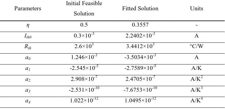
Nonlinear unconstrained optimization problems are considered to solve the model parameters. In this paper, we use the simplex method. First, we can set the initial feasible solution x(0)=(η,Ith0,Rth,a0,a1,a2,a3,a4) which is shown in Table 1. Then according to the optimization theory

(whether the target condition is satisfied), we can determine whether the solution is feasible. If satisfied, calculation stops and the solution is obtained; if it is not satisfied, new feasible solution x(n)=(η,Ith0,Rth,a0,a1,a2,a3,a4) n=1,2…n should be produced from the current solution. The new

feasible solution will be closer to the target condition, and then they will be judged according to the target condition, which forms the iterative algorithm. In this way, iterative solutions are constantly improved until the target condition is satisfied. Finally, the fitted model parameters can be obtained [3]. The target condition in this paper is:

|𝑓(𝑥)| < 𝜀 (𝜀 tends to 0)

𝑓(𝑥) = 𝑃0 − 𝜂[𝐼 − 𝐼𝑡ℎ0− ∑4𝑛=0𝑎𝑛(𝑇0+ (𝐼𝑉 − 𝑃0)𝑅𝑡ℎ)𝑛]. (6)

By using the simplex method, the parameters are searched by iteration. After 1073 iterations, we put the current feasible solution into function f(x). The value is 8.59×10-5, which meets the target condition. The fitted solution of model parameter (η,Ith0,Rth,a0,a1,a2,a3,a4)is shown in Table 1.

Table 1. Initial feasible solution and fitted solution of parameters for LI curves.

Parameters Initial Feasible

Solution Fitted Solution Units

η 0.5 0.3557 -

Ith0 0.3×10-3 2.2402×10-3 A

Rth 2.6×103 3.4412×103 °C/W

a0 1.246×10-3 -3.5034×10-3 A

a1 -2.545×10-5 -2.7589×10-5 A/K

a2 2.908×10-7 2.4705×10-7 A/K2

a3 -2.531×10-10 -7.6753×10-10 A/K3

a4 1.022×10

-12

Comparison to Experiment

Take the above fitted parameter values into Eq. 5, we can get the LI curves. But there is still a variable V in Eq. 5. To solve this problem, we can fit the current-voltage (IV) experimental data by using a polynomial function of current. And there we choose six terms. So the fitted curve can be expressed as follows:

𝑉 = 1.400 + 0.4424𝐼 − 0.105𝐼2+ 1.425 × 10−2𝐼3− 9.150 × 10−4𝐼4+ 2.233 × 10−5𝐼5. (7) Where the unit of current is mA. Besides, the comparison between the fitted curve and the experimental values is shown in Fig. 1. And it can be seen that the curve fits well. The LI curve can be finally got by combining the optimal model parameters with Eq. 5 and Eq. 7.

Figure 1. Comparison of experimental and fitted IV curve at 20°C.

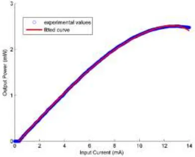
Fig. 2 illustrates the comparison of experimental and the fitted LI curves at the ambient temperature of 20°C. It is can be seen that the model shows good agreement. However, there is a certain deviation between them within the range of 13mA to 14mA.

Figure 2. Comparison of experimental and fitted LI curve at 20°C.

Model Improvement

To improve the model accuracy, we employ the following two approaches：

(1) Change the highest order of polynomial for fitting IV curve and choose seven terms instead to improve the precision. The IV fitted curve can be expressed as:

(2) It is more appropriate to consider a relationship of a resistance in series with a diode in some cases on the basis of the structure of the VCSEL to fit IV curve. The diode-like relationship is as follows:

𝑉 = 𝐼𝑅𝑆+ 𝑉𝑇𝑙𝑛 (1 + 𝐼

𝐼𝑠). (9)

Where Rs is the serial resistance, VT and Is are the diode’s thermal voltage and saturation current

respectively. VT can be treated as a constant at a certain temperature. To fit the Eq. 9, we should get

the values of Rs, VT and Is.

In the same way, we employ the simplex method. On the basis of the experimental IV data, we can get the parameter values when the target condition is met after several iterations: Rs=5.7877×10-2, VT=0.1501 and Is=9.700×10-6. So the IV data at 20°C can be fit using the following relationship:

𝑉 = 5.7877 × 10−2𝐼 + 0.1501𝑙𝑛 (1 + 𝐼

9.700×10−6). (10)

Where the unit of current is mA.

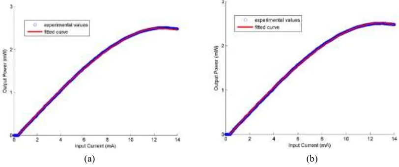
These two methods are respectively combined with the optimal model parameters and Eq. 5 to draw the LI curve at 20°C. The comparison between the fitted and experimental values is shown in Fig. 3. It is can be seen that the fitted values are in good agreement with the experimental values after the two methods of improvement. Especially for methods (2), it improves a lot within the range of 13mA to 14mA.

(a) (b)

Figure 3. Comparison of experimental and the improved fitted curve (a is based on the method 1; b is based on the method 2).

To further analyze the accuracy of the model, we use Root Mean Square Error (RMSE), Normalized Mean Bias (NMB) and Normalized Mean Error (NME) as model evaluation index. RMSE is used to measure the deviation between the experimental and the fitted values. NMB and NME reflect average deviation and mean absolute error. Besides, NMB and NME are close to 0, which shows that the fitting effect is good. The expressions for RMSE, NMB, and NME are as follows:

𝑅𝑀𝑆𝐸 = √1

𝑁∑(𝑦

∗_{− 𝑦)}2 ₍₁₁₎

𝑁𝑀𝐵 =∑(𝑦∗−𝑦)

∑ 𝑦 × 100% (12)

Table 2. Model evaluation index.

RMSE NMB/% NME/%

Simulated

LI curve 0.0159 -0.1876 0.6656 Improved curve

(Method 1) 00152 -0.2692 0.6965

Improved curve

(Method 2) 0.0144 -0.1288 0.6462

As is seen from the Table 2, compared to the not improved model and the improved model based on the method (1), the model evaluation index of the improved model based on the method (2) are closer to 0. Through analysis, we can see that the improved LI curve by using method (2) has better fitting effect.

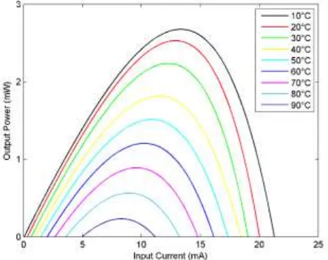
Furthermore, we apply better improved model to draw the LI curves in the ambient temperature range 10-90°C, as is shown in Fig. 4. We can conclude that the maximum value of the output power decreases as the ambient temperature increases.

Figure 4. LI curves in the ambient temperature range 10-90°C.

Conclusions

In this paper, the simplex method is used in parameter estimation to simulate the LI characteristics of VCSEL. In order to increase the accuracy of the model, we improve the way to fit the IV data. The model evaluation index is introduced to compare with the experimental value. The index reveals that it is more appropriate to fit the IV data using the relationship which accounts for a resistance in series with a diode. Furthermore, the improved model can be applied to fit the LI curves at different ambient temperatures, and it illustrates that maximum value of the output power decreases as the ambient temperature increases.

Acknowledgement

This research was financially supported by the National Science Foundation of China (Grant No. 41775039, 41775165, and 91544230).

References

[2] Liu J, Gao J, Li Y. Rate-Equation-Based VCSEL Thermal Model and Simulation, C. Environmental Electromagnetics, the 2006, Asia-Pacific Conference on. IEEE, 2006:139-143.