Electricity Consumption Prediction Using XGBoost Based on Discrete Wavelet Transform

2017 2nd _{International Conference on Artificial Intelligence and Engineering Applications (AIEA 2017)}

ISBN: 978-1-60595-485-1

Electricity Consumption Prediction Using XGBoost

Based on Discrete Wavelet Transform

WEIZENG WANG, YULIANG SHI, GAOFAN LYU and WANGHUA DENG

ABSTRACT

The purpose of this paper is to predict the daily electricity consumption of the next month. It is considerably important for people to cope with the problem well. Although few articles mentions the topic of electricity consumption prediction, numerous papers include some topic similar to the topic in this paper, such as rainfall forecasting, wind speed prediction and water flow forecasting. Moreover, a number of techniques and algorithms are employed to cope with those issues and achieve outstanding performance. Those techniques and algorithms are considerably remarkable, but the accuracy of them is not excellent enough on the long-term prediction of time series. In this paper, we propose a hybrid model which integrate discrete wavelet transform and XGBoost to forecast the electricity consumption time series data on the long-term prediction, namely DWT-XGBoost. The original time series data can decompose into approximate time series data and detail time series data by the discrete wavelet transform. And those time series data by decomposition are as features input into the prediction model that is XGBoost. Furthermore, the parameters of XGBoost are obtained by a grid search method. The performance of the proposed model in this paper is measured against with other hybrid models such as integrating discrete wavelet transform and support vector regression, integrating discrete wavelet transform and artificial neural networks, and unitary XGBoost. The comparison results show that the DWT-XGBoost outperforms other models and is a novel method on the long-term prediction of time series.

KEYWORDS

Wavelet Transform, Discrete Wavelet Transform (DWT), XGBoost, DWT-XGBoost, Extracting Features.

INTRODUCTION

At present, people cloud not live a better life without electricity, and it is considerable essential to distribute electricity effectively and protect power supply demand. It requires data scientists to rely on effective analysis methods and accurate forecasting models of electricity demand, and to develop the history of electricity records to accurately predict the next period of electricity consumption and explore the electricity law of the actual world. The record of electricity here is a time series. _________________________________________

Corresponding Author: Weizeng Wang,[email protected], Beijing University of Technology, People’s Republic of China.

On the time series prediction, the most popular method is the statistical the ARMA at before, followed by the emergence of machine learning and deep learning.

In machine learning, many researchers have developed many single or hybrid models for time series prediction, which have been validated in actual data. Ye Ren used a novel hybrid model of integrating the EMD (empirical mode decomposition) and the SVR to predict wind speed in his study, then compared with a variety of hybrid models and finally found that the hybrid model proposed by himself was more accurate [1]. In the study of fault time series prediction, Xin Wang and Ji Wu proposed a hybrid model of singular spectrum analysis and the SVR, compared with various models such as the ARMA and multiple linear regression, and found that the performance of the model in this example was better than those models [2]. Adamowski and Sun compared the relative performance of the coupled wavelet-neural network models (WA–ANN) and regular artificial neural networks (ANN) for flow forecasting at lead times of 1 and 3 days for two different non-perennial rivers in semiarid watersheds of CyprusR, found that the performance of the former was better [3]. Similarly, Venkata Ramana and others haven combined the wavelet transform with ANN to obtain a hybrid model named WNN, and regular ANN and it were then applied to monthly rainfall prediction respectively to gain a conclusion that the prediction accuracy of the latter is better than that of the former [4]. And before that, a scholar has put forward an approach of nonlinear SVM based on PSO (particle swarm optimization algorithm) applied to rainfall forecasting as well [5]. Zhiyong Liu and others investigated a hybrid model that was combined the discrete wavelet transform and support vector regression (the DWT– SVR model) for daily and monthly stream flow forecasting and found it outperformed regular SVR [6]. In addition, some other hybrid models and unicity models for forecasting have also been proposed, such as AGA-SSVR which hybridizes SVR model with adaptive genetic algorithm (AGA) and the seasonal index adjustment [7], Recurrent Neural Networks(RNN) and Grammatical Inference [8], the least squares support vector regression [9,10], SVR or SVM [11,12,13,14], Neural Networks [15]. Most of the above are only developed to short-term time series prediction. Moreover, other investigators have made some results in long-term time series prediction. Alexander Grigorievskiy and others applied OP-ELM to the problem of long-term time series prediction [16]. Multiple-output support vector regression (M-SVR) have been employed in multi-step-ahead time series prediction by Yukun Bao and others [17]. The least squares support vector machine and the multivariate adaptive regression spline model are applied to the long-term prediction of river water pollution by Ozgur Kisi et al [10].

can accurately predict the future electricity situation. And the forecasting results can provide decision support for the power sector so that are enable them to more effectively configure the power to avoid uneven distribution. The major contribution of this paper is as follows: 1) the introduction of related work, 2) describing the hybrid model proposed in this paper 3) describing experiment procedure, 4) discussing results, 5) the final part of the conclusion.

RELATED WORK

This section provides brief introductions to the related techniques including extreme gradient boosting (XGBoost), discrete wavelet transform (DWT), and grid search used in the hybrid model. In this paper, XGBoost is used to model the fluctuation, while DWT is used to decompose the electricity consumption time series.

EXTREME GRADIENT BOOSTING (XGBOOST)

XGBoost is short for “Extreme Gradient Boosting”, where the term “Gradient Boosting” is proposed in the paper Greedy Function Approximation: A Gradient Boosting Machine, by Friedman [19]. XGBoost is based on this original model. This is a machine learning method that has been used by many data researchers, especially in a variety of data competitions and machine learning competitions, reflects the performance of more superior than other methods. The XGBoost is applicable in both classification and regression, which has been validated in many practical cases, such as store sales prediction, customer behavior prediction, ad click through rate prediction, hazard risk prediction, web text classification, malware classification [18].

XGBoost is used for supervised learning problems, where we use the training data (with multiple features) xi to predict a target variable yi. As described by Chen and Guestrin [18], Xgboost is an ensemble of K Classification and Regression Trees (CART) {T1 (xi, yi)... TN (xi, yi)} where xi is the given training set of descriptors associated with a molecule to predict the class label, yi. Given that a CART assigns a real score to each leaves (outcome or target), the prediction scores for individual CART is summed up to get the final score and evaluated through K additive functions, as shown in Eq. 1:

y_i= fk(xi) K

k=1 ,fk∈F. (1)

Where Kthe number of trees is, fk is a function in the functional spaceF, and F is the

space of all CART. And the objective function contain two parts: training loss and regularization, as shown in Eq. 2:

obj θ = l y_i,y_i

n

i

+ Ω(fk) K

k=1

. (2)

Since additive training is used, the prediction y_i at step t expressed as

y_i(t)= fk K

k=1

xi =yi (t-1)

+ft xi . (3)

And tree boosting is used to Eq. 2, it can be written as

obj θ (t)= l y_i,y_i(t-1)+ft(xi) n

i

+Ω ft . (4)

After a series of improvements and evolutions, Eq. 5 is derived, which is used to score a leaf node during splitting.

Gain= 1 2

GL2

HL+λ+

GR2

HR+λ

-GL+GR 2

HL+HR+λ -γ (5)

Where the first, second and third term of the equation stands for the score on the left, right and the original leaf respectively. Moreover, the final term, γ, is regularization on the additional leaf.

The most important factor behind the success of the XGBoost is its scalability in all scenarios. The scalability of XGBoost is due to several important systems and algorithmic optimizations. These innovations include: a new tree learning algorithm for dealing with sparse data; theoretically reasonable weighted quintile sketch program can handle instance weights in approximate tree learning. Parallel and distributed computing makes learning faster, enabling faster model exploration [18]. Although the XGBoost is based on the classification and regression tree (CART) and the gradient boosting, XGBoost is better than them because it integrates both the advantages.

DISCRETE WAVELET TRANSFORM (DWT)

The discrete wavelet transform (DWT) is one of the wavelet analysis. In here, wavelet is a mathematical function that represents the scale of time series and their relationship to analyze time series that contain non-stationaries. The advantage of wavelet analysis is that it allows the use of long time intervals for low-frequency information and shorter intervals for high-frequency information and is capable of revealing aspects of data like trends, breakdown points, and discontinuities that other signal analysis techniques might miss. Another is that the mother wavelet can be flexibly selected according to the characteristics of the time series investigated. Wavelet analysis contain two approaches: the one is the continuous wavelet transform (CWT), another is the discrete wavelet transform (DWT).

The definition of the continuous wavelet transform is as fallow

CWTxΨ τ, s = 1_|

s| x t Ψ

* t-τ

s dt

+∞

-∞ (6)

noted here that the CWT calculations require a lot of time and resources [3]. In addition, the CWT generates a lot of data, which contains a lot of redundant information, which will lead to more difficult data analyses [6]. However, the DWT is simpler to implement than the CWT and requires less computation time. Even so, it`s analysis is still very effective and accurate [3, 6]. The DWT scales and positions are usually based on integer powers of two (dyadic scales and positions) [6]. This is achieved by modifying the wavelet transform function representation to

Ψj, k t-γ

s =

1 s0

j 2⁄ Ψ

t-kγ₀s0 j

s₀j (7)

Where Ψ is the wavelet function, t is the time and γ is the translation factor (time step) of the wavelet over the time series, s indicates the scale (scale factor), j is an integer that determines the dilation (dilation factor), k is an integer that determines the translation, s0 is a specified fixed dilation step greater than 1, and γ0 denotes the location

parameter which must be greater than 0.

DWT decomposes the original waveform into two waveforms by two complementary filters (high frequency and low frequency): the approximate waveform (A) and the detail waveform (D). The approximate waveform is a high-scale and low-frequency component; the detail waveform is a low-scale and high-low-frequency component. It is generally believed that the low frequency approximate waveforms are representative of the original waveform of the same, and the high-frequency detail waveforms represent subtle changes in the original waveform, so either of them is indispensable. The DWT process is an iterative decomposition. If the number of decomposed layers is greater than 1, then the decomposition of the approximate waveform begins from the second layer. So an original waveform after DWT decomposition will produce a lot of high-frequency detail waveforms, and only a low frequency approximation waveform.

Performance Criteria

The performance of each model is verified by using different statistical measures. The statistical measures used in this study are: mean square error (MSE) and correlation coefficient (R). The mean square error is defined as fallow

MSE 1

N yi-yi

2 N

i=1

(8)

Where Nthe number of data points is, y_i is the observed value, y_i is the calculated value. The definition of correlation coefficient is fallow

R ∑ yi-yi

N

i=1 yi-yi

∑ _y

i-yi 2 N

i=1 ∑ yi-yi 2 N

i=1

(9)

THE DWT-XGBOOST BASED HYBRID MODEL

In the above section, DWT and XGBoost have been briefly introduced. This section describes DWT-XGBoost used in this study, and because of integrating DWT with XGBoost, it is called DWT-XGBoost.

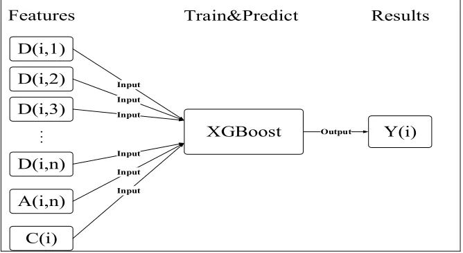
At present, the researchers have not published papers on the combination of them. In this study, the main content of that is using DWT to decompose the original time series and then obtaining the set of sub-series which are as features input to the XGBoost model outputting results finally. The DWT-XGBoost model construction shown in Figure 1. Some researchers believed that the set of sub-series by DWT decomposition needed to use some reliable selection method to select the more appropriate sub-series as features [6], but some others indicated that all sub-series should be used as features and are equally important, because each sub-series are derived from the original time series [3]. In this study the latter's argument is adopted. The Hybrid model can be expressed as Eq. 10

Yi XGBoost Di,1,Di,2, ⋯ ,Di,n,Ai,n,Ci 10

Where Di,n represents the n-the decomposition layer of detail waveform,

Ai,n represents the n-the decomposition layer of approximate waveform, and Ci

represents other factors.

In this study, a month is generally within five weeks, therefore five models corresponding to five weeks are trained. There are progressive relationships between five models, and the weekly predictive values obtained from the previous forecasting are used to construct feature sets for the later. The definition of that is as follow

Fi=f0+∑i-1j=0gj, i ∈1,2,3,4,5 (11)

Where Fi represents the itch model, f0 represents the initial influencing factor (ie, the

feature set has not been added to the predicted value construct), g represents the influencing factor from predictive values of the j-the model, and g is 0.

D(i,1)

D(i,2)

D(i,3)

D(i,n)

· ·

· XGBoost

Input Input Input

Input

A(i,n)

Input

Y(i)

Output

Features Train&Predict Results

C(i)

Input

EXPERIMENTS

Dataset

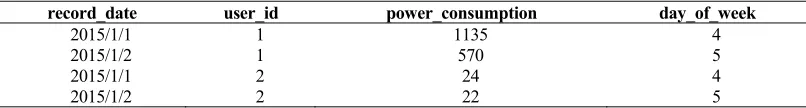
The data used in this study is the statistics of the historical power consumption of all enterprises on Yangzhong High-tech Industrial Development Zone of Jiangsu Province, China, and provided by Tianchi Big Data Competition hosted by Ali Cloud. Table 1 shows the historical data format. The forecast is the total daily electricity consumption of the next month for all enterprises in the region.

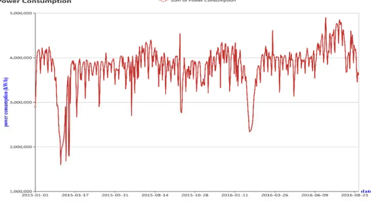
After preliminary statistical analysis, it is found that the total daily electricity consumption shows a periodicity, week as a unit, as shown in Fig. 2. Due to the existence of some legal holidays in China, there are also some specific high and low peak segments, but the overall trend is presented in weekly units. Although forecasting the total daily electricity consumption is final objective, the overall trend is reflected in the daily electricity consumption for each enterprise. The historical power consumption of each enterprise is employed for training and forecasting after processing, then the prediction values will be counted up, finally we will count the total daily electricity consumption next month. Because of the periodicity nature and the long-term prediction, it is considered to divide original time series into different sub-time series according to everyday of a week, in which each enterprise is corresponding to seven kinds of sub-time series. Consequently, original prediction goal transforms into forecasting the electricity consumption of each enterprise on next some days in the same period. Before doing the above, we need to fill missing values. And for some reason, there are no electricity records for some enterprises someone day. Due to small amount of the missing, it is probably reasonable that the missing is set 0 value. After initially processing, the new data format is got, as shown in Table 2. And there is an attribute, day_of_week (its values consist of 1 to 7), which corresponds to date (e.g.: 4(Thursday) corresponds 2015/1/1(January 1, 2015)).

TABLE 1. THE HISTORICAL DATA FORMAT.

record_date user_id power_consumption

2015/1/1 1 1135

2015/1/2 1 570

2015/1/1 2 24

2015/1/2 2 22

TABLE 2 ADDING DAY_OF_WEEK AFTER PROCESSINGRECORD_DATE.

record_date user_id power_consumption day_of_week

2015/1/1 1 1135 4

2015/1/2 1 570 5

2015/1/1 2 24 4

Figure 2. The total daily electricity consumption from 2015-01-01 to 2016-08-30.

Features Extraction

The section describes tow methods of features extraction, basic statistics and wavelet transform. We employ these features extracted by the above of methods in prediction stage.

Features Extraction Based on Basic Statistics

This section describes how to use basic statistics to extract features. Here we use the mean and standard deviation statistic to construct features from the time series. After dividing into train sets

And test sets by the time period, the part of each set used to construct features is calculated fallowing the statistics. Following the day_of_week attribute hardly, the average and standard deviation of the electricity consumption per enterprise can be obtained from subsets within the entire range of that set. And then according to the day_of_week, absolutely, the average and standard deviation of that can also be calculated from subsets within one day in the same period of the entire range of that set. As shown Table 3, where user_id denotes enterprise ID, DOW_power_mean is mean of the electricity consumption according to the day_of_week, DOW_power_std is standard deviation of that according to the day_of_week, power_mean is mean of that not fallowing the day_of_week, power_std is standard deviation of that not fallowing the day_of_week. In addition, all records presenting fluctuations haven potential information in the same period, they are also as features. As shown Table 4, where 1_week denotes first day of the same period, the rest are similar.

Features Extraction Based On Wavelet Transform

decomposing them using the discrete wavelet transform of wavelet transform. There are some of the configuration parameters on the DWT need be set: the parent wavelet is db2 in Daubechies wavelets; according to the length of subsets, the number of decomposition layers is 2; the edge expansion function using zero- padding. Binding the above configuration parameters to the DWT, and then that is employed decomposition, obtaining sub-wavelets of time series as features. As shown Table 5, where w0 denotes one value of someone of sub wavelets, the rest are similar. Moreover, it is very important to keep all means and standard deviations of the upper section as features.

Note: where the attributes user_id and day_of_week are not used for training.

TABLE 3. THE FEATURES OF MEAN AND STANDARD DEVIATIONS. user_i

d day_of_week DOW_power_mean DOW_power_ power_std power_mean

1 1 312.9167 84.59149 98.75397 307.0595

1 2 316.9167 102.2523 98.75397 307.0595

TABLE 4. ALL RECORD DATA OF THE SAME PERIOD.

user_id day_of_week 1_week 2_week 3_week ···

1 1 393 354 328 ···

1 2 35 341 462 ···

TABLE 5. THE FEATURES OF SUB-WAVELETS BY DECOMPOSITION OF THE DISCRETE WAVELET TRANSFORM.

user_id day_of_week w0 w1 w2 _· ··

1 1 -60.52715344 480.229347 633.6039154 _· ··

1 2 -55.22629175 341.5180818 708.8183392 _· ··

TABLE 6. THERE ARE THE LIST OF CANDIDATE PARAMETERS CORRESPONDING TO THE FEATURE SET OBTAINED BY THE WAVELET TRANSFORM EXTRACTING FEATURES,

OPTIMAL PARAMETER SET AND BEST SCORE ABOUT GENERAL -XGBOOST.

Best Parameters _Best

Score

n_estimators objective learning_rat_e max_delta__step max_dep_th

150 reg:tweed_ie 0.15 1 3 0.97671₉₆₂

150 reg:tweed_ie 0.15 1 5 0.95426₃₁₁

200 reg:tweed_ie 0.10 1 2 0.87063₆₅₃

200 reg:gam_ma 0.10 1 3 0.85799₉₉₇

200 reg:tweed_ie 0.10 1 2 0.83683₈₀₉

Candidate parameters

{50, 100, 150, 200}

{reg:linea r, reg:gam

ma, reg:tweed

ie}

{0.05, 0.10,

0.15} {1}

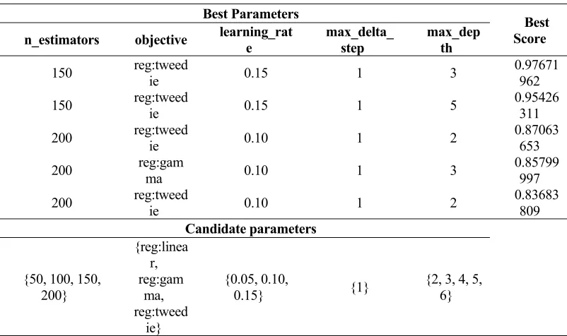
TABLE 7. THERE ARE THE LIST OF CANDIDATE PARAMETERS CORRESPONDING TO THE FEATURE SET OBTAINED BY THE WAVELET TRANSFORM EXTRACTING FEATURES,

OPTIMAL PARAMETER SET AND BEST SCORE ABOUT DWT-XGBOOST.

Best Parameters _Best

Score

n_estimators objective learning_rat_e max_delta__step max_dep_th

200 reg:tweed_ie 0.15 1 5 0.99062₉₈₃

200 reg:tweed_ie 0.15 1 5 0.98932₄₆₃

150 reg:tweed_ie 0.15 1 2 0.95832₆₉₂

150 reg:tweed_ie 0.15 1 2 0.94573₂₂₉

150 reg:tweed_ie 0.1 1 3 0.95506₈₄₅

Candidate Parameters

{50, 100, 150, 200}

{reg:linea r, reg:gam

ma, reg:tweed

ie}

{0.05, 0.10,

0.15} {1} {2, 3, 4, 5, 6}

Modeling Process

Once feature sets are constructed, models are constructed. The prediction model used in this study is XGBoost, and its parameters need to be set manually. In training phase, the GridSearchCV (cross-validated grid-search) is applied to select these parameters in the sclera toolkit of Python [2]. It is, to some extent, preventive that the accuracy of the prediction model decreases due to using the parameters set by subjective assumptions to train models [6]. After using the selection method, the optimal set of parameters in the candidate parameters are sought out. It is important to note here that the time spent in this selection process increases as the amount of training data increasing. In this study, the feature datasets are used for selecting an optimal parameter set for training prediction model, repeating the procedure can obtain all models. There only show the modeling process about regular XGBoost namely General-XGBoost and DWT-XGBoost, in order to highlight advantage of XGBoost in train stage. And they are shown in Tables 6 and 7 respectively, where n_ estimators is the number of boosted trees to fit the actual scene, objective is the learning task and the corresponding learning objective, learning rate is learning rate, max_delta_step is maximum delta step, max_depth is maximum tree depth.

RESULTS AND DISCUSSIONS

Model Performance

Before discussion, Table 6 and 7 need be explained. And it is very obvious from the Best Score in the two tables that the training score of DWT-XGBoost is superior to that of General-XGBoost. From the two models, scores of each model show a decreasing trend, which indicates the characteristics of long-term prediction accuracy attenuation that can be also reflected in the following analysis.

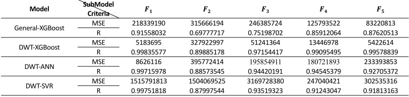
At the training phase, two statistical metrics, mean square error (MSE) and correlation coefficient (R), are employed to validate all models. As shown in Table 8 that contains the MSE and R values for each kind of model. In order to indicate clearly the difference between all models, these MSE and R values are plotted into the parallel coordinate map, which they are respectively shown Fig. 3 and Fig. 4. As can be seen from Fig. 3, the MSE value of DWT-XGBoost model is significantly smaller than that of other three models. But the MSE value of DWT-XGBoost is slightly larger than that of General-XGBoost at , which may be due to the fact that the data used for verification corresponds to an especial period in the actual scene. And the phenomenon cannot affect the generalization of model. As can be seen from Fig. 4, the R value of DWT-XGBoost model is also significantly larger than1 that of other three models. Moreover the R value of the former is basically close to 1. We find out that DWT-SVR is very well about its R value, but its MSE value is largest in all models from Fig. 3. In addition, the R value of General-XGBoost is lowest in Fig. 4.

At the forecasting phase, the same two statistical metrics were used before. As shown in Table 9, MSE and R values are calculated from the statistical summary of predicted values and observed values which is by the competition. While MSE and R values of the forecasting phase are calculated from the predicted and observed values of each model. As can be seen from Table 9, MSE and R of DWT-XGBoost are significantly better than that of other three models. In particular, MSE and R of DWT-SVR are not presented, because the differences of it and other three models are too large.

Model Prediction Results

All model are applied to predict the daily electricity consumption for each company in the next month respectively, then that results aggregate the total daily electricity consumption for a month. As we can see from Fig. 5, predicted values of DWT-SVR differ greatly from those of other three models and observed values. Except from DWT-SVR, predicted values of other three models and observed values are shown in Fig. 6. And we can find that predicted values of DWT-XGBoost are closer to observed values, which is obvious to compare with other two models. The above suggests that not only DWT-XGBoost outperform other three models (DWT-ANN, DWT-SVR and General-XGBoost) about accuracy but also the generalization ability of it is better.

TABLE 8. DURING TRAINING PHASE, THERE ARE MSE AND R ON FOUR MODELS.

Model  SubModel 

Criteria           

General‐XGBoost  MSE  218339190  315666194  246385724  125793522  83220813 

R  0.91558032  0.69777717  0.75198702  0.85912064  0.87620513 

DWT‐XGBoost  MSE  5183695  327922997  51241364  13446978  5422614 

R  0.99835577  0.89885178  0.97154417  0.99095495  0.99578839 

DWT‐ANN  MSE  8626116  395772414  195854911  180721893 233393853 

R  0.99715978  0.88573545  0.94420191  0.94545379  0.92705372 

DWT‐SVR  MSE  1515791813  1504069525  3169728380  247040421  302535316 

TABLE 9. DURING FORECASTING PHASE, THERE ARE MSE AND R ON THREE MODELS.

Model  MSE  R 

General‐XGBoost  771482693043  ‐0.43225086 

DWT‐XGBoost  113920387382  0.32561234 

DWT‐ANN  782352782056  0.29163273 

Figure 3. MSE values in training phase.

Figure 5. The compare of predicted values and observed values (four models).

CONCLUSION

Comparing with the four models in the above statement, DWT-XGBoost in the respect of time series prediction shows superiority. This study is to apply this model to electricity consumption forecast. In the future, if we have the opportunity we will apply it to other fields, and will continue to improve the model. For time reasons, we still have improved requirements in some places. For example, in the data section, we can add weather data and regional economic data, and use the cross validation method to segment the data set. In the algorithm section, we can use more candidate combinations of parameters. Of course, the more the combination of the parameters, the more the training time.

ACKNOWLEDGEMENTS

Corresponding Author: Weizeng Wang, Beijing University of Technology, People’s Republic of China. [email protected].

REFERENCES

1. Ren, Y., Suganthan, P.N., & Srikanth, N. A novel empirical mode decomposition with support vector regression for wind speed forecasting. IEEE transactions on neural networks and learning systems, 27(8) (2016) 1793-1798.

2. Wang, X., Wu, J., Liu, C., Wang, S., & Niu, W. A Hybrid Model Based on Singular Spectrum Analysis and Support Vector Machines Regression for Failure Time Series Prediction. Quality and Reliability Engineering International, 32(8) (2016) 2717-2738.

3. Adamowski, J., & Sun, K. Development of a coupled wavelet transform and neural network method for flow forecasting of non-perennial rivers in semi-arid watersheds. Journal of Hydrology, 390(1) (2010) 85-91.

4. Ramana, R.V., Krishna, B., Kumar, S.R., & Pandey, N.G. Monthly rainfall prediction using wavelet neural network analysis. Water resources management, 27(10) (2013) 3697-3711.

5. Vikram, P., & Veer, P.R. Rainfall forecasting using nonlinear svm based on pso. IJCSIT) International Journal of Computer Science and Information Technologies, 2 (2011) 2309.

6. Liu, Z., Zhou, P., Chen, G., & Guo, L. Evaluating a coupled discrete wavelet transform and support vector regression for daily and monthly streamflow forecasting. Journal of hydrology, 519(2014) 2822-2831.

7. Chen, R., Liang, C.Y., Hong, W.C., & Gu, D.X. Forecasting holiday daily tourist flow based on seasonal support vector regression with adaptive genetic algorithm. Applied Soft Computing, 26 (2015) 435-443.

8. Giles, C.L., Lawrence, S., & Tsoi, A.C. Noisy time series prediction using recurrent neural networks and grammatical inference. Machine learning, 44(1) (2001) 161-183.

9. Yuan, C., Xu, S., & Zhang, X. Prediction of water quality base on kernel clustering least squares support vector regression. In Control, Automation, Robotics and Vision (ICARCV), 2016 14th International Conference on (pp. 1-5). IEEE.

10. Kisi, O., & Parmar, K.S. Application of least square support vector machine and multivariate adaptive regression spline models in long term prediction of river water pollution. Journal of Hydrology, 534(2016) 104-112.

11. Wu, C.H., Ho, J.M., & Lee, D.T. Travel-time prediction with support vector regression. IEEE transactions on intelligent transportation systems, 5(4) (2004) 276-281.

12. Sapankevych, N.I., & Sankar, R. Time series prediction using support vector machines: a survey. IEEE Computational Intelligence Magazine, 4(2) (2009).

13. Yang, H., Chan, L., & King, I. Support vector machine regression for volatile stock market prediction. Intelligent Data Engineering and Automated Learning—IDEAL 2002(2002) 143-152.

14. Müller, K.R., Smola, A., Rätsch, G., Schölkopf, B., Kohlmorgen, J., & Vapnik, V. Using support vector machines for time series prediction. Advances in kernel methods—support vector learning, (1999) 243-254.

15. Frank, R.J., Davey, N., & Hunt, S.P. Time series prediction and neural networks. Journal of Intelligent & Robotic Systems, 31(1) (2001) 91-103.

16. Grigorievskiy, A., Miche, Y., Ventelä, A.M., Séverin, E., & Lendasse, A. Long-term time series prediction using OP-ELM. Neural Networks, 51(2014) 50-56.

17. Bao, Y., Xiong, T., & Hu, Z. Multi-step-ahead time series prediction using multiple-output support vector regression. Neurocomputing, 129(2014) 482-493.

18. Chen, T., & Guestrin, C. Xgboost: A scalable tree boosting system. In Proceedings of the 22nd acm sigkdd international conference on knowledge discovery and data mining (pp. 785-794), (2016, August). ACM.