2016 6th International Conference on Information Technology for Manufacturing Systems (ITMS 2016) ISBN: 978-1-60595-353-3
An Adaptive Disturbance Model for Model Predictive Control
Liguo Zhang
College of Automation, Chongqing University, Chongqing, China
ABSTRACT: This paper proposes an adaptive disturbance model for the modeling and estimation of unmeasured disturbances. The residuals generated as a result of the output error of the process model, are used to model the unmeasured disturbances at the output. A two-stage recursive least-squares (TSRLS) algorithm is derived for the online estimation of the disturbance model parameters. The proposed scheme is capable of estimating both the stationary and non-stationary disturbances. The adaptive disturbance model is used in a model predictive control (MPC) technique to provide improved disturbance rejection. The future behavior of the modeled disturbances is predicted and incorporated into the model predictions to improve their accuracy. The effectiveness of the proposed approach is shown by the simulation example of a glasshouse process.
KEYWORDS: Model predictive control; Adaptive disturbance model; Parameter estimation; Disturbance rejection
1. INTRODUCTION
Model predictive control is the most widely applied advanced control technique in the process industries. MPC uses the plant model to predict its behavior over a certain time horizon. At each time interval, a cost function is minimized to optimize the future behavior of the plant. MPC has shown improved results when applied on a multi-input multi-output (MIMO) system and has become an important tool for dealing systems with constraints. Since MPC is a model based technique, its performance is highly dependent upon the kind of process model used. Due to the plant-model mismatch, which is very common in a real-time environment, control performance of the whole system can degrade. The models like finite impulse response (FIR) and step response models were used in early MPC algorithms like the dynamic matrix control (DMC) [1] and the quadratic DMC (QDMC) [2]. Generalized predictive control (GPC) by Clark et al. [3] used transfer function based approach. Most of the works done recently in MPC area use the state space formulations. State space based MPC techniques have also been used in some industrial MPC tools [4].
Due to the presence of unmeasured disturbances in the system, target tracking becomes very difficult to achieve. It is required to properly model these unmeasured disturbances so that their effects can be included in the MPC formulations. The linear quadratic regulator used a constant state disturbance model [6]. The DMC and QDMC used an output
step disturbance model. Using a fixed disturbance model shows degraded performance when the disturbances in the system are time varying. These unmeasured disturbances are required to be efficiently modeled and require some online identification technique for their modeling and estimation. This is lead to the development of adaptive MPC techniques. One of the widely used adaptive MPC techniques is the GPC. Gencili and Nikoloau [9] proposed an MPC and identification (MPCI) approach, in which an on-line optimization problem is solved. Shen and Lee [10] presented an auto regressive model for representing unmeasured disturbances. Karra et al. [11] presented a MPC based technique in which both the process and disturbance models are updated in real time by using two separate recursive regression schemes. Xu et al. [12] proposed an adaptive disturbance model based on a multi-iteration pseudo-linear regression scheme. A Kalman filter based tuning for improved disturbance rejection was presented by Gerksic et al. [13]. Muske and Badgwell [14] underlined the conditions necessary to achieve offset free control by adding constant disturbance models either at output or at state or both. Pannocchia and Rawlings [15] proposed a general disturbance model using an unstructured model.
most of the disturbances in industries are nonstationary. These disturbances are caused by change in room temperature, material composition, flow rates etc The general characteristic of the non-stationary disturbances is that they are time varying, so are difficult to be modeled. The modeling of non-stationary disturbances is a complex task because of their time varying nature and they cannot be represented by a certain structure. Generally, the unmeasured disturbances are represented as filtered white noise and their dynamics are defined by some autoregressive or moving average autoregressive models. In [3] and [12], an integrated white noise based disturbance model is used to represent the non-stationary disturbances, a difference operation is used their representation which results in stationary description. To properly capture all the dynamics of disturbances, a disturbance model is required which can capture the effects of both the stationary and non-stationary disturbances. In this work an adaptive disturbance model for an MPC scheme is proposed, in which both the stationary and non-stationary unmeasured disturbances are estimated online. The stationary disturbances are represented by an ARMA model and the non-stationary disturbances are represented by a time-varying bias term. In the MPC scheme, the plant model remains fixed while the parameters of the disturbance model are estimated online using the TSRLS algorithm. In the adaptive disturbance model identification, no test signals are required so it is free from persistent excitation issues.
Based on the decomposition schemes of [17] and [18], a TSRLS algorithm is derived for the online parameter estimation of the adaptive disturbance model. The TSRLS algorithm allows separate parameter estimation for the stationary and non-stationary disturbances with different forgetting factors and covariance matrices. The TSRLS algorithm provides accurate estimates and is capable of estimating the effects of non-stationary disturbances. The proposed adaptive disturbance model can be used with any MPC techniques. In this work, we will use the adaptive disturbance model to modify an MPC scheme based on the non-minimal state space (NMSS) process model with a constant output disturbance. The predicted disturbance values, from the adaptive disturbance model are included in the model predictions to improve their accuracy. By using the proposed adaptive disturbance model we will only modify the prediction part of the MPC scheme based on the NMSS model.
This paper is organized as follows: Section 2 briefly reviews the MPC approach using the NMSS model. Section 3 presents our proposed adaptive disturbance model and the TSRLS algorithm. In section 4, efficiency of the proposed scheme is illustrated with example of a glasshouse process. Section 5 is the conclusion.
2. MPC WITH A CONSTANT OUPUT
DISTURBANCE
One of the most popular ways to deal with unmeasured disturbances in an MPC scheme is to add a constant output disturbance in the process model. This scheme is widely used in process control industries.
2.1.System Representation
Let the plant with ( )u t as its the input and ( )y t
as its output be described by the following discrete time transfer function:
1 1
( ) ( ) ( )
( )
H q
y t u t
F q
−
−
= (1)
Where
1 1 2
1 2
( ) 1 f
f
n n F q− = + f q− + f q− +L+ f q− ,
1 1 2
1 2
( ) h
h
n n H q− =h q− +h q− +L+h q− ,
Are polynomials in unit backward shift operator
1
q− (i.e., 1 ( ) ( 1)
q u t− u t = − ),
f
n and nh represent
the orders of polynomials ( 1)
F q− and H q( −1)
respectively.
Remark 1:
For simplicity, the single-input single output (SISO) is considered here, while extension to multi-input multi-output (MIMO) is straightforward and only requires few notational modifications.
The state vector is selected as
( )T [ ( ), , ( 1), ( 1), , ( 1)]
f h
x t = y t K y t n− + u t− Ku t n− +
The NMSS space model is defined in the following manner [5]:
( ) ( 1) ( 1)
( ) ( )
x t Ax t Bu t y t Cx t
= − + −
= (2)
Where
1 2 2
1 0 0 0 0
0 1 0 0 0
0 0 0 0 0
0 0 0 1 0
0 0 0 0 0
f h
n n
f f f h h
A
− − −
=
L L
L L
L L
M M O M M O M
L L
L L
M M O M M O M
L L
[
1 0 1 0 0]
T
B = h K
[
1 0 0 0 0]
C= K
as the state variables. So, it does not require the use of any observer which is generally required by most of the state space based techniques. By avoiding the use of observer, it is free from observer based issues like convergence rate and robustness of the overall system.
2.2. Prediction and Control
The NMSS model is generally used in MPC scheme with a constant output disturbance model, which is described as [4]
( 1) ( ) ( )
( 1) ( )
( ) ( ) ( )
x t Ax t Bu t d t d t
y t Cx t d t + = + + =
= +
(3)
In which ( )d t represents the output disturbance.
The disturbance is estimated as ( )d t = y t( )−Cx t( ). For defining the model predictions, the future state and control vectors are represented as
( | ) ( 1| ), ( 2 | ), , ( p| ) T
x t t% =x t+ t x t+ t K x t+N t
(4)
[
]
( | ) ( | ), ( 1| ), , ( 1| )T c
u t t% = u t t u t+ t K u t+N − t (5)
( | ) ( 1| ), ( 2 | ), , ( p| ) T
y t t% =y t+ t y t+ t K y t+N t (6)
( | ) ( 1| ), ( 2 | ), , ( p| ) T
d t t% =d t+ t d t+ t K d t+N t (7)
Where Np is the prediction horizon and Nc is
the control horizon. The future state values are described as
( | ) ( ) ( | )
x t t% =Fx t + Φu t t% (8)
Where
2 3
p
N
A A A F
A
=
M
, 2
1 2 1
0 0
0 0
p p p c
N N N N
B
AB B
A B AB
A − A − B A − − B
Φ =
L L L
M M O M
L
The future model outputs are defined as
( | ) ( | ) ( | )
y t t% =Cx t t% +d t t% (9)
Where C N( P×((nf +nh)×Np)) is a Np-block diagonal matrix having matrix C from (2) on its diagonal. Since ( 1)d t+ =d t( ) , d t t%( | ) could be expressed as
[
]
( | ) ( ) ( ) 1
p
N
d t t% = y t −Cx t (10)
Where 1
p
N is a vector containing Np number of 1’s. Hence, the future output values are expressed as
[
]
( | ) ( | ) 1 ( ) ( )
p
N
y t t% =Cx t t% + y t −Cx t (11)
For computing the optimal control moves over a finite prediction horizon, the following cost function is minimized:
0 1 0
( ( ) ( | )) ( ( ) ( | ))
( ( | )) ( ( | ))
p
c
M
T
sp sp
j
N
T
i
J y j y t j t Q y j y t j t
u t i t R u t i t =
−
=
= − + − +
+ + +
∑
∑
(12)
Subject to
min max
min max
( )
( )
u u t j u y y t j y
≤ + ≤ ≤ + ≤
Where yap is the future set-point vector, Q and
R is positive definite weighting matrices on the output and the control signal, respectively. umin
and umaxare the limits for the control signal. ymin
and ymaxare the limits for the output signal. The
optimization problem in (12) can be solved by means of quadratic programming, using the well-known techniques.
3. MPC WITH ADAPTIVE DISTURBANCE
MODEL
The constant output disturbance model of (10) is not capable of capturing the dynamics of unmeasured disturbances in the system. In this section we will derive a TSRLS algorithm for estimating parameters of the adaptive disturbance model. From the estimated disturbance model, future values of the disturbances are predicted and added to the output predictions of (9) to improve their accuracy. In the proposed scheme only the prediction part of the MPC scheme described in the last section is modified while the optimization part remains unchanged.
Assuming that we have a negligible plant-model mismatch, then unmeasured disturbance at the output could be estimated as
ˆ( ) ( ) ˆ( )
d t = y t −y t (13)
Where ˆ( )y t is the model output. We are
considering that both stationary and non-stationary disturbances are present in the system. So, the dynamics of the estimated disturbance can be described as
ˆ( ) ˆ( ) ˆ( )
d t =w t +η t (14)
time-varying bias term representing the non-stationary disturbances. The dynamics of the stationary disturbances are described as an ARMA process in the following manner:
1 1
ˆ ( , )
ˆ ( ) ( )
ˆ ( , )
C q t
w t e t
D q t −
−
= (15)
Where ( )e t is white noise with zero mean and
finite variance. The model order of the ARMA process is calculated using the final prediction error approach. The parameters of the disturbance model in (14) are estimated using the TSRLS algorithm. 3.1. Two stage RLS algorithm
The combined disturbance effect of both stationary and non-stationary part is described as
1 1
ˆ ( , )
ˆ( ) ( ) ˆ( )
ˆ ( , )
C q t
d t e t t
D q t
η
−
−
= + (16)
The decomposition scheme divides the system into different subsystems which results in improved accuracy in the parameter estimation. One important feature of the decomposition technique is that it can be used for systems where different parameters have different characteristics with respect to time or some other variable. The model in (16) cannot be identified using a (one-stage) RLS algorithm, because it contains a time-varying part
η
ˆ( )t and a time-invariant part ˆ ( )w t . The TSRLS algorithmallows separate parameter estimation for the stationary and nonstationary components of the disturbance model with different forgetting factors and covariance matrices. Equations (15) can also be expressed as
1 2
1
ˆ ˆ ˆ
ˆ( ) ( ) ( 1) ( ) ( 2) ( ) ( )
ˆ ˆ
( ) ( ) ( 1) ( ) ( )
d
c
n d
n c
w t d t w t d t w t d t w t n e t c t e t c t e t n
= − − − − − −
+ + − + + −
K K
(17) For defining (17) in standard regression form, we define the parameter vectors
θ
ˆ ( )1 t andθ
ˆ ( )2 t as1 ˆ1 ˆ2 ˆ 1 2
ˆ( ) ( ), ( ), , ( ), ( ), ( ), ,ˆ ˆ ˆ ( )
d c
c d
T
n n
n n
t d t d t d t c t c t c t
θ
+
=
∈ℜ
K K
(18)
2
ˆ( )t ˆ( )t
θ
=η
(19)Equation (17) contains unmeasurable variables
( )
w t−i and (e t−i), these unknown variables are
replaced by their estimates ˆ (w t−i) and ˆ(e t−i),
respectively. The information vectors
φ
ˆ ( )1 t and 2ˆ ( )t
φ
are defined as1
ˆ( ) [ ˆ( 1), ˆ( 2), , ˆ( ),
ˆ( 1), (ˆ 2), , (ˆ )] c d
d
n n
T d
t w t w t w t n
e t e t e t n φ
+
= − − − − − −
− − − ∈ ℜ
K K
(20)
2
ˆ ( ) 1t
φ
= (21)The augmented parameter and information vectors are defined as
1 1
2
ˆ ( ) ˆ( )
ˆ ( ) c d
n n
t t
t θ θ
θ
+ +
= ∈ ℜ
(22)
1 1
2
ˆ ( ) ˆ( )
ˆ ( ) c d
n n
t t
t φ φ
φ
+ +
= ∈ ℜ
(23)
From (14), we have
1 1 2 2
ˆ( ) ˆ( ) ˆ( ) ˆT( ) ( )ˆ ˆT( ) ( )ˆ ( )
d t =w t +
η
t =φ
tθ
t +φ
tθ
t +e t . (24) The model in (24) is our identification model for the system in (14). For the system decomposition, we first define the following two intermediate variables:1 2 2
ˆ( ) ˆ( ) ˆT( ) ( )ˆ
d t =d t −
φ
tθ
t (25)2 1 1
ˆ ( ) ˆ( ) ˆT( ) ( )ˆ
d t =d t −
φ
tθ
t (26)From (25) and (26), the system in (24) can be decomposed into the following two subsystems:
1 1 1
ˆ( ) ˆT( ) ( )ˆ ( )
d t =
φ
tθ
t +e t (27)2 2 2
ˆ ( ) ˆT( ) ( )ˆ ( )
d t =
φ
tθ
t +e t (28)The loss function for each of the two subsystems is defined as
2
1
ˆ
ˆ ˆ
( ( )) t t j[ ( ) T( ) ( )] , 1, 2.
i i i i i i
j
J θ t λ − d j φ jθ t i =
=
∑
− = (29)Where λ is the forgetting factor which is
introduced to cater the estimate of time varying term. From (29), the recursive least squares algorithm for computing
θ
ˆ ( )i t is defined by the following set of equations:1
ˆ
ˆ( ) ˆ( 1) ( )[ ( ) ˆ ( ) ( 1)],ˆ
ˆ ˆ ˆ
( ) ( 1) ( )[ ( ) ( 1) ( )] ,
1 ˆ
( ) [ ( ) ( ) ( 1)],
1, 2.
T
i i i i i i
T
i i i i i i i
T
i i i i
i
t t K t d t t t
K t P t t t P t t
P t I K t t P t
i
θ θ φ θ
φ λ φ φ
φ λ
−
= − + − −
= − + −
= − −
=
(30)
Substituting (25) and (26) into (30), with i= 1, 2 respectively,
θ
ˆ ( )i t is estimated as1 1 1 ˆ 2 2 1 1
ˆ( ) ˆ( 1) ( )[ ( ) ˆ ˆT ( ) ˆ ˆT ( 1)]
t t K t d t t t
θ
=θ
− + −φ θ
−φ θ
−(31)
2 2 2 ˆ 1 1 2 2
ˆ( ) ˆ( 1) ( )[ ( ) ˆ ˆT ( ) ˆ ˆT ( 1)]
t t K t d t t t
θ
=θ
− + −φ θ
−φ θ
−By replacing the unknown parameter vectors
1
ˆ ( )t
θ ,θˆ ( )2 t in (31)-(32), with their preceding
estimates
θ
ˆ ( 1)1 t− andθ
ˆ ( 1)2 t− , respectively, wehave
1 1 1 2 2 1 1
1 1
ˆ
ˆ( ) ˆ( 1) ( ) ( ) ˆ ˆ( 1) ˆ ˆ( 1)
ˆ
ˆ( 1) ( ) ( ) ˆ ( ) ( 1)ˆ
T T
T
t t K t d t t t
t K t d t t t
θ θ φ θ φ θ
θ φ θ
= − + − − − −
= − + − −
(33)
2 2 2 2 2 2 2
2 2
ˆ
ˆ( ) ˆ( 1) ( ) ( ) ˆ ˆ( 1) ˆ ˆ( 1)
ˆ
ˆ( 1) ( ) ( ) ˆ ( ) ( 1)ˆ
T T
T
t t K t d t t t
t K t d t t t
θ θ φ θ φ θ
θ φ θ
= − + − − − −
= − + − −
(34)
The gains are defined as
1 1( ) 1( 1) ( )ˆ1 1 ˆ1 ( ) (1 1) ( )ˆ1
T
K t p t φ t λ φ t P t φ t −
= − + − (35)
1 2( ) 2( 1) ( )ˆ2 2 ˆ2( ) (2 1) ( )ˆ2
T
K t p t φ t λ φ t P t φ t −
= − + −
(36)
And the covariance matrices are defined as
1 1 1 1
1
1 ˆ
( ) ( ) ( ) ( 1)T
P t I K t φ t P t λ
= − − (37)
2 2 2 2
2
1 ˆ
( ) ( ) ( ) ( 1)T
P t I K t φ t P t λ
= − − (38)
The inner variables are calculated as
ˆ ˆ
ˆ ( ) ( ) ( )
w t =d t −η t (39)
1 1
ˆ ˆ ˆ( ) ˆ( ) T( ) ( )
e t =w t −
φ
tθ
t (40)For the TSRLS algorithm, the initial values of the covariance matrices are selected as 1(0) 0
c d
n n
P = p I + ,
andP2(0)= p0, where p0 is selected as a large
number ( 6
0 10
p = ). The parameter estimates
θ
ˆ (0)1and
θ
ˆ (0)2 are chosen as 1nc+nd /p0 and1/p0 ,respectively, where 1m is a vector with m numbers of 1’s in it. The important point in the parameter selection is the forgetting factor λifor the two
subsystems. For the stationary noise model ( ˆ ( )w t ),
we selectλ1=1, giving equal weight to all the data.
For the time varying bias term, we consider it as a time-varying part of the output disturbance, which does not have a fix mean or a variance. For this reason,λ2 is used as a tuning parameter for to
obtaining greater accuracy, which could be defined as [21]
2 2
2
( ) 1
1 ( ) e
e t P t λ
σ = −
+
Where σe is the disturbance variance. The
TSRLS algorithm for computing ˆ( )θ t and ˆ( )φ t is
summarized in the following steps: 1) P1(0) p I0 na+nb
= , 2(0) 0
c d
n n
P = p I + , P3(0)= p0 ,
1 0
ˆ (0) 1 /
a b
n n p
θ = + ,
θ
ˆ (0) 1/2 = p0, 6 0 10p = , ˆ ( ) 0w i = ,
ˆ( ) 0
e i = for i≤0.
2) Estimated the output disturbance from (13) and form
φ
ˆ ( )1 t by (20) andφ
ˆ ( )2 t by (21)3) Compute K t1( ) by (35) and K t2( ) by (36)
4) Compute P t1( ) by (37) and P t2( ) by (38)
5) Update the parameter estimates θˆ ( )1 t by (33) and θˆ ( )2 t by (34)
6) Compute ˆ ( )w t by (39) and ˆ( )e t from (40)
Step 2-6 are repeated at each sampling instant. 3.2.Disturbance predictions
The identified stationary noise model ˆ ( )w t is
represented as
1 2
1
ˆ ˆ ˆ
ˆ( ) ( ) ( 1)ˆ ( ) (ˆ 2) ( ) (ˆ )
ˆ( ) ˆ( ) ( 1)ˆ ˆ ( ) (ˆ )
d
c
n d
n c
w t d t w t d t w t d t w t n e t c t e t c t e t n
= − − − − − −
+ + − + + −
K K
The state vector for the stationary noise model is defined as
[
ˆ ˆ ˆ]
( )T ( ), , ( 1), ( ), , ( 1)
n d c
x t = w t K w t−n + e t K e t−n +
and the time-varying state space model is defined as
( ) ( ) ( 1) ( ) ( )
ˆ ( ) ( ) ( )
n n n n
n n
x t A t x t B t e t w t C t x t
= − +
= (41)
Where
1( ) 2( ) ( ) 1( ) ( )
1 0 0 0 0
0 1 0 0 0
( ) 0 0 0 0 0
0 0 0 0 0
0 0 0 1 0
0 0 0 0 0
c d
n n
n
c t c t c t d t d t
A t
− − −
=
K K
K K
K K
M M O M M O M
K K
K K
K K
M M O M M O M
K K
[
]
( )T 1 0 0 0 1 0 0
n
B t = K
[
]
( ) 1 0 0 0 0 0 0
n
C t = K
The output of the NMSS model in (3) with estimated disturbance model is expressed as
ˆ ˆ
( ) ( ) ( ) ( )
y t =Cx t +w t +
η
t (42)( ( )w t ) and a time-varying bias term ( ( )η t ). The
proposed adaptive MPC scheme is illustrated inFig. 1. For the prediction of disturbances, we define the following future vectors:
( | ) ( 1| ), ( 2 | ), , ( | )
ˆ ˆ ˆ
( | ) ( 1| ), ( 2 | ), , ( | )
ˆ ˆ ˆ
( | ) ( 1| ), ( 2 | ), , ( | )
ˆ ˆ ˆ
( | ) ( 1| ), ( 2 | ), , ( | )
T
n n n n p
T
p
T
p
T
p
x t t x t t x t t x t N t
w t t w t t w t t w t N t
e t t e t t e t t e t N t
t t t t t t t N t
η η η η
= + + +
= + + +
= + + +
= + + +
% K
% K
% K
% K
(43)
( ) y t ( )
w t η( )t
sp y
ˆ( )
y t d tˆ( )
+ −
( ) u t
( | ) y t t%
Figure 1. Schematic of the MPC with adaptive disturbance model.
The future disturbance states of the stationary noise model are defined as
( | ) ( ) ( | )
n n n n
x t t% =F x t + Φ e t t%
Where
2 3
( ) ( ) ( )
( ) p
n
n
n n
N n
A t A t A t F
A t
=
M
, 2
1 2
( ) 0 0
( ) ( ) ( ) 0
( ) ( ) ( ) ( ) 0
( ) ( ) ( ) ( )
p p
n
n n n
n n n n
n
N N
n n n n
B t
A t B t B t A t B t A t B t
A − t A − t B t B t
Φ =
K
K
K
M M O M
K
Since we have assumed ( )e t to be zero mean
white noise, its future values will be approximately equal to its mean, i.e.
( | ) 0
e t t% =
Hence, we have the future stationary disturbance values defined as
( | ) n n( | ) n n n( )
w t t% =C x t t% =C F x t (44)
Where Cn (Np×((nc+nd)×Np)) is a Np-block
diagonal matrix having matrix Cn from (41) on its
diagonal.
η
ˆ( )t is assumed to remain constant throughout the prediction horizonˆ ( | ) ( )1
p
N
t t t
η
% =η
(45)The future disturbance values are now defined as
( | ) n n n( ) ( | )
d t t% =C F x t +η% t t (46)
By using (2) as the process model and (46) representing the predicted disturbances, the model predictions in (11) can be redefined as
( | ) n( | ) n n n( ) ( | )
y t t% =Cx t t% +C F x t +η% t t (47)
From (47) and (11), it can be seen that, instead of having constant output disturbances, the predicted values of disturbances are included in model predictions to improve their accuracy. Furthermore, these disturbances include effects of the both stationary and non-stationary disturbances which results in improved prediction quality.
4. SIMULATION EXAMPLE
In this section, MPC scheme with an adaptive disturbance model will be represented as AMPC, while the MPC with constant output disturbance model will be represented simply as MPC.
4.1.Glasshouse Process
For a multi-input multi-output (MIMO) system with constraints, a simulation example of a glasshouse process is presented. The process can be explained by the following dynamics [19]
1
1 1
1 1
1
2 1 2
1
0.015 0.077
( ) 1 0.905 ( )
( ) 0.058 ( )
0.753 1 0.793
q
q
y t q u t
y t q u t
q q
−
− −
−
− −
−
−
=
−
−
−
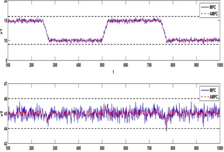
Figure 3. Close-loop output responses using the MPC and the AMPC schemes.
[image:7.612.63.296.229.387.2]Figure 4. Close-loop control signals for MPC and AMPC schemes.
Table 1. The estimated parameters for the adaptive disturbance model using TSRLS algorithm. Estimation
Algo. t c1 d1 Error(%)
TSRLS 500 -0.3194 0.2601 7.8
1000 -0.3615 0.2252 2.98
1500 -0.3668 0.2536 3.06
2000 -0.3734 0.2385 1.10
3000 -0.3751 0.2212 0.63
True Values -0.39 0.22
Where y t1( ) and y t2( ) are the air temperature
and the relative humidity of the air respectively.
1( )
u t and u t2( ) are valve aperture of boiler and
spraying input respectively. The model in NMSS form is represented as
( 1) ( ) ( )
( ) ( )
x t Ax t Bu t y t Cx t
+ = + =
Where
0.905 0 0 0.07
0 0.793 0 0.0597
0 0 0 0
0 0 0 0
A
−
=
0.015 0.077
0.058 0.753
1 0
0 1
B
−
−
=
, 1 0 0 0
0 1 0 0
C=
It is required to keep the air temperature between 16 and 9(9≤ y t1( ) 16)≤ and relative humidity is to
be maintained at 45% with 2% variation allowed
2
(44.2≤ y t( ) 45.8)≤ . u t1( )is allowed to change
between 30% and 35% (30≤u t1( ) 35)≤ and
second input u t2( ) is allowed to change between 6% and 11% (6≤u t2( ) 11)≤ . For the MPC design
4 c
N = and 100
p
N = . Weights on both error and
control signal identity matrices. Both of the outputs are affected by the following stationary and the non-stationary disturbances:
1 1
( )
( ) ( )
( )
C q
w t e t
D q −
−
= ,
( ) 0.05sin(0.02 ) 0.12sin(0.09 )t t t
η = + .
Where
1 1
( ) 1 0.932
C q− = − q− ,D q( −1) 1 0.28= + q−1,
And ( )e t is the zero mean white noise with
variance σ2=0.102. Fig. 3 shows output responses
with constraints. Fig. 4 shows input responses with constraints. Fig. 2 shows that by using the TSRLS algorithm is able to capture the dynamics of the non-stationary disturbance. Because of having an additional term for representing the non-stationary disturbances, the adaptive disturbance model provides a better estimate for unmeasured disturbances. It is clear from the responses that both MPC and AMPC are able to meet the required constraints. Due to the adaptive disturbance model in the AMPC it was able to reject the disturbances more rapidly. The integrated absolute error (IAE) value for both systems is calculated as
1000 2 1 1
( ) ( )
i spi
k i
IEA y k y k
= =
=
∑ ∑
−The IAE value of MPC is 153.41 and that of AMPC is 132.85, that is 14% less than the MPC.
5. CONCLUSIONS
[image:7.612.53.301.449.552.2]adaptive disturbance model was used in a MPC scheme with a fixed process model. The predicted disturbance values were incorporated into model predictions to improve their accuracy. The effectiveness of the proposed work was illustrated through the example of a glasshouse process.
REFERENCES
[1]C.R. Cutler, B.L. Ramaker. Dynamic matrix control-a computer control algorithm, AICE national meeting, 1979. [2]C.E. Garcia, A.M. Morshedi. Quadratic Programming
solution of dynamic matrix controlv (QDMC). Chemical Engineering Communications, vol. 46, pp. 73–87, 1986. [3]D.W. Clarke, C. Mohtadi, P.S. Tuffs. Generalized
predictive control. Part 1: the basic algorithm. Part 2: extensions and interpretations. Automatica, vol. 23, no. 2, pp. 137–160, 1987.
[4]S.J. Qin, T.A. Badgwell. A survey of industrial model predictive control technology. Control Engineering Practice, vol. 11, no. 7, pp.733–764, 2003.
[5]C.L. Wang, P.C. Young. An improved structure for model predictive control using non-minimal state space realisation. Journal of Process Control, vol. 16, no. 4, pp. 355–371, 2006.
[6]H. Kwakernaak, R. Sivan. Linear Optimal Control Systems. John Wiley & Sons, 1972.
[7]M. Morari, J.H. Lee. Model predictive control: the good, the bad, and the ugly. Proceedings of the Fourth International Conference on Chemical Process Control, pp. 419–444, 1991.
[8]M.C. Wellons, T.F. Edgar. The generalized analytical predictor for chemical process control. Industrial Engineering Chemical Research, vol. 26, no. 8, pp. 1523-1536, 1987.
[9]H. Genceli, M. Nikolaou. New Approach to Constrained Predictive Control with Simultaneous Model Identification. American Institute of Chemical Engineers Journal, vol. 42, no. 10, pp. 2857–2867,1996.
[10] G.C. Shen, W.K. Lee. A predictive approach for adaptive inferential control. Computer and Chemical Engineering, vol. 13, no. 6, pp.687–701, 1989.
[11] S. Karra, R. Shaw, S.C. Patwardhan, S. Noronha. Adaptive model predictive control of multivariable time-varying systems. Industrial Engineering Chemical Research, vol. 47, no. 8, pp. 2709–2720, 2008.
[12] Z. Xu, Y. Zhu, K. Han, J. Zhao, J. Qian. A multi-iteration pseudolinear regression method and an adaptive disturbance model for MPC. Journal of Process Control, vol. 20, no. 4, pp. 384–395, 2010.
[13] S. Gerksic, S. Strmcnik, Ton van den Boom. Feedback action in predictive control: an experimental case study. Control Engineering Practice, vol. 16, no. 3, pp. 321–332, 2008.
[14] K.R. Muske, T.A. Badgwell. Disturbance modeling for offset-free linear model predictive control. Journal of process Control, vol. 12, no. 5, pp. 617–632, 2002.
[15] G. Pannocchia, J.B. Rawlings. Disturbance model for offset-free model predictive control. American Institute of Chemical Engineers Journal , vol. 49, no. 2, pp. 426–437, 2003.
[16] L. Ljung. System identification: Theory for User, 2nd Edition, Pearson Education, 1998.
[17] F. Ding, H. Duan. Two-stage parameter estimation algorithms for Box-Jenkins systems. Signal Processing, IET, vol. 7, no. 8, pp. 646-654, 2013.
[18] R. Ding, H. Duan. TS-RLS algorithm for pseudo-linear regressive models. American Control Conference (ACC), Montreal, Canada, pp. 2683-2688, 2012.
[19] P.C. Young, M.J. Lee, A. Chotai, W. Tych, Z.S. Chalabi. Modelling and PIP control of a glasshouse micro-climate. Control Engineering Practice, vol. 2, no. 4, pp. 591–604, 1994.
[20] L. Ljung, T. Soderstrom. Theory and practice of recursive identification, The MIT Press, 1983.