Locating Total Domination Number in Strong Product of Two Paths

2019 International Conference on Computational Modeling, Simulation and Optimization (CMSO 2019) ISBN: 978-1-60595-659-6

Locating-Total Domination Number in Strong Product of Two Paths

Kang WEI, Jian-ping LI and Zhe-min LI

College of Liberal Arts and Sciences, National University of Defense Technology, Changsha, Hunan 410073, China

Keywords: Locating-total domination, Strong product, Path.

Abstract. In a monitoring system, each node's status is unique, and the system can accurately locate the node when there is a problem, which can be modeled through graphs’ locating-total domination. When laying out the monitoring system, it is crucial to select the root node. Given a graph G, its locating-total domination number is the minimum cardinality of G’s locating-total dominating set. In this paper, we give the bounds of this number for the strong product of two paths.

Introduction

Considering the problem of monitor placement in a monitoring system, each node (consisting of the monitoring device) is linked to the monitor and is modeled by graphs’ total-domination. If someone goes wrong in the system, it will be located by the monitor uniquely, which can be simulated by the graph’s locating-total domination. When laying out the monitoring system, we need to consider many factors, such as the cost and the work efficiency of the system, how to select the root node is crucial.

The study on graphs’ locating-dominating set of was pioneered by Slater [1-3], which has been extended to total domination. Locating-total domination in graphs was firstly studied by Haynes et al.[4], which has been further studied in References [5-10].

Given a simple connected graph G with a vertex set ( )V G and an edge set ( )E G . Denote the open neighborhood of a vertex v by N v( ), which is the set of vertices linking to it. Denote the closed neighborhood of v by N v[ ], which is { }v N v( ). Given a subset S V G( ), we defined the

open neighborhood of S as N(S)_v_SN(v) , and defined the closed neighborhood as

] [ ]

[S N v

N _v_S .Given an S, if every vertex in ( )V G is adjacent to at least one of its vertex, then S

is a total dominating set. Such S is a locating-total dominating set if N(u)S  N(v)S. Here, this set is abbreviated as LTD-set. A graph with no isolated vertex contains a LTD-set. Denoted the locating-total domination number of G by r_tL(G). It is the minimum cardinality of G’s

locating-total dominating set.

The strong product of two simple graphs is mentioned in References[11,12]. Given two simple connected graphs G and H, we denoted their strong product by G H. Two vertices ( , )g h_{i i} and

(g h_j, _j) ofV G( H) connect to each other if and only if they satisfy one of the following conditions:

1. g_i g_iandh h_{i j}E H( ),

2.g g_{i j}E G( ) andh_i h_i,

3.g g_{i j}E G( )and h h_{i j}E H( ).

Let S be a subset of ( )V G .All the edges of G with all endpoints in S consists of the edge set. This obtained subgraph of G is called the derived subgraph of S in G. Let B be a subset of ( )E G , and its vertex set is composed of all the vertices of G that are associated with at least one edge in B. Taking

B as the edge set, the derived subgraph of G is called the edge derived subgraph of B in G.

Denote a path with n vertices by P_n. The strong product of two paths P_mand P_nis denoted by

m n

P P. In [2], Haynes and Henning showed that ( )

     

L t P

We derived the bounds for the locating-total domination number ofP_m P_n. We use v_ijto denote

the vertex in (V P_m P_n), where 1im, and 1 jn. Let S be a LTD-set ofP_m P ._n Define that

) n j 1 }( , , ,

{ 1 2   

 j j mj

j S v v v

S  , and |S_j| is the vertex number of S_j. Besides, EC refers to the columns which exclusive vertex in S.

Locating-Total Domination Number of P₂ P_n

We calculated the locating-total domination number ofP₂ P_n.

Theorem 1.If n3, r P_tL( ₂ P_n)n.

Proof. Let S {v_1i|i1,3,5}{v_2j| j2,4,6}(see Fig.1).

One can check that S is a LTD-set ofP₂ P_n, and |S|=n. Thusr_tL(P₂ P_n)n.

Figure 1. A LTD-set of P₂ P_n.

Assume that r_tL(P₂ P_n)n, there is|S_i| 0 for some i with1in. Since N v[ ]_1i N v[ _2i]and

1i, 2i

v v S , then N(v_1i)S N(v_2i)S , it is inconsistent with the definition of LTD-set, so

2

( )

L

t n

r P P n.

Based on the analysis above, L( ₂ )

t n

r P P n.

Locating-Total Domination Number of P₃ P_n

We calculated the locating-total domination number ofP₃ P_n. Theorem 2. If n3, L( ₃ ) ₉n

t n

r P P    n _{ }.

Proof. If n is odd, S{v_1i|i2,4,6, ,n1}{v_2j| j1,3,5, ,n}.

If n is even, S{v12,v21}{v2i|i4,6,8, ,n}{v3j | j3,5,7, ,n1}(see Fig.2).

It is not difficult to check that S is a LTD-set of P₃ P_n, and S n. Thus r_tL(P₃ P_n)n.

Figure 2. A LTD-set ofP3 Pn.

Let S be a LTD-set of P₃ P_n . Therefore, |S_i1||S_i||S_i1|0 ,where 2in1 . When 0

| | |

|S_i  S_i1  , we break up the graph between column i and column i1, then columns i andi1

are viewed as boundary columns. The graphP₃ P_n is divided into several parts, and none of them

contain|Si ||Si₁|0. Those parts can be viewed as new graphs.

Conjecture 1: When |S_i| 0( 2  i n 1), then there exist positive integers p and q, such that

2

i p

The purpose is to allow columns that do not contain vertex in S can borrow vertex in S from columns that contain two or more vertex in S. The proof is completed by considering the three cases:

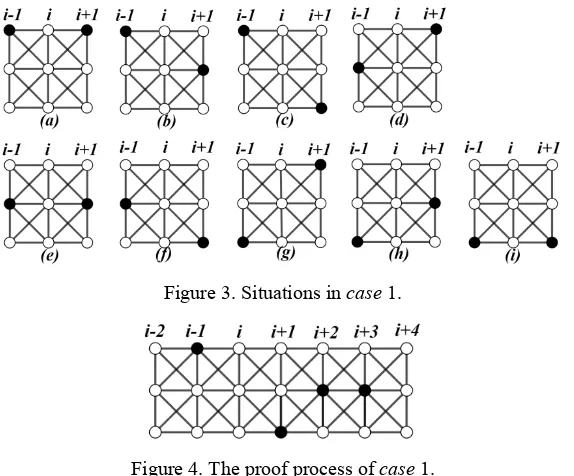
Case 1. S_i 0, S_i1 1, S_i1 1.

All the situations have been list in Fig.3. By the definition of LTD-set, it is easy to prove that those are not true except situations in Fig.2c and Fig.2g. Without loss of generality, we focus on the right side of Fig.2c (see Fig.4).

Figure 3. Situations in case 1.

Figure 4. The proof process of case 1.

In Fig.4, if S_i2 2, the conjecture holds. By the definition of LTD-set, we take S_i2 1, it

clear thatv2(i2)S . Since v1(i1)S v1(i2)S andv2(i1)S v3(i2)S , we get Si3 1 and

S

v2(i3) . If Si3 2 , the conjecture holds. Otherwise, Si3 1, and Si3 {v2(i3)}. Since

S v

S v

S

v_1(i₂₎  _1(i₃₎  _3(i₃₎ , we can get Si4 2.

Obviously, for case 1, the conjecture holds.

Case 2. S_i 0, S_i1 3, S_i1 1, or S_i 0, S_i1 1, S_i1 3.

The column i can borrow a vertex in S from column i-1 or columni+1, it does not affect the integrity of the conjecture.

Case 3. S_i 0, S_i1 2, S_i1 1, or S_i 0, S_i1 1, S_i1 2.

Without loss of generality, we focus onS_i 0, S_i1 2, S_i1 1.

All the situations have been list in Fig.5, it is no difficult to check that situations in

Fig.5a,5b,5c,5d are unreasonable by considering the vertices in column i. Situations in

Fig.5e,5f,5g,5h can be proved the same way as the situation in Fig.4.

For the situation shown in Fig.5i, it is clear that S_i2 1. We assumed that S_i2 {v_1(i2)}. Since

S v

S

v_3(i1)  _3(i2) , we get S_i3 1 . If S_i3 1 , S_i3 {v_2(i3)} .When it appears another

EC(column i+k) closest to column i from the right side, than S_{i x} 1 1





Figure 5. Situations in case 2.

Since |Si₁||Si₂| |Sik₁|1 , N(v1i)Si1N(v2i)Si1 N(v3i)Si1 ,and

1 )

( 3 1

) ( 2 1

) (

1 ) ( ) ( )

(v ik Sik  N v ik Sik  N v ik Sik

N    ,the column i and the column i+k can be

viewed as boundary columns that split off the column from i1 to i k 1.

Based on the analysis above, G is divided into as many parts as possible. All the EC in G are either boundary column of these parts or can borrow a vertex in S from columns that contain two or more vertices in S. In addition, if the boundary column is EC, the adjacent column must have two or more vertices in S. For each part, n' is defined as the number of columns, S'is this subgraph’s locating-total dominating set. Obviously, only if both boundaries of this subgraph are EC and there is another EC in the subgraph, that |S' |can be less thann'and one EC cannot borrow vertex in S

from the left or right sides. Besides, it is not difficult to prove that if |S₁| 0 , then |S₂| 2 , and if

2 2

S  , then S₂ {v₁₂,v₃₂}. When |S_n| 0 , the same as |S₁| 0 .In this case, S'  n' 1. Now we

want to find the minimum value of n'.In Fig.6, it is clear that S₃ {v₂₃} and S₇ {v₂₇}.Base on the proof in case 1,when both boundary of this subgraph are EC and there exist another EC, it is easy to prove that n' 9 . In Fig.7, we show the case when n' 10 and n' 11 . As the subgraph in Fig.6 and Fig.7, several subgraphs of P₃ P₃can be added (see Fig.7c). Therefore, when 9 n' 17, it

can always take S'  n' 1.

Based on the analysis above, we divide G as many as possible into the subgraph which n'= 9,

therefore, ( 3 ) 9

L n

t n

r P P    n _{ }.

Figure 6. A LTD-set of P₃ P₉.

Figure 7.n'could be 10 to 17, such that S' n' 1 .

Locating-Total Domination Number of P₄ P_n

Theorem 3. If n4, n 1 r_tL(P₄ P_n) n 2.

Proof. If n is odd, S{v₄₁,v_4n}{v_2i |i1,3,5,,n}{v_3j | j2,4,6,,n1}. If n is even, S{v₄₁,v_1n}{v_2i |i1,3,5,n1}{v_3j | j2,4,6,,n} (see Fig.8).

One can find that S is a LTD-set of P₄ P_n, and S  n 2. Obviously, r P_tL( ₄ P_n) n 2.

Figure 8. A LTD-set of P₄ P_n.

Now we discuss the lower bound of r_tL(P₄ P_n). Let S be P₄ P_n’s LTD-set. There is no i such that |Si₁||Si||Si₁|0. For|Si||Si1|0, we break up the graph between columns i andi+1,

which can be both viewed as boundary columns of their respective parts.

When S_i 0, it easy to prove that S_i1 and S_i1 cannot both equal to 1 with 2  i n 1. In fact, conjecture 1can be used here as well. We proved the conjecture the two cases:

Case 1. S_i 0, S_i1 2, S_i1 1, or S_i 0, S_i1 1, S_i1 2.

Without loss of generality, we focus on S_i 0, S_i1 2, S_i1 1.

All the situations have been list in Fig.9. It's easy to prove that situations in

Fig.9a,9b,9d,9g,9h,9i,9j do not conform to the definition of LTD-set by considering the neighbor of the gray vertices. For situations in Fig.9c,9f, if S_i2 1, it cannot be true by considering the

neighbor of the gray vertices(see Fig.10a,10b). Therefore, Si2 2. For the situation inFig.9e, we

have Si2 1, if Si2 1, thenv3(i1)S , it is clear that Si3 2(see Fig.10c). Therefore, the

conjecture holds.

Figure 9. Situations in case 1.

Case 2. S_i 0, S_i1 3, S_i1 1, or S_i 0, S_i1 1, S_i1 3.

The column i can borrow a vertex in S from column i1 or columni1, it does not affect the integrity of the conjecture.

When S₁ 0 or S_n 0, it is not difficult to prove that S₂ 3 or S_n1 3.

Therefore, once the graph appears EC, column which contains three or more vertices in S that appear on the left or right sides, or columns which contain two or more vertices in S that appear on the left and right sides. In this way, the locating-total domination number of each part is at least one more than its column number, thus is |S|n+1.

If there is no EC in G. When S1 1and S2 1, there are only two cases, that are {v21,v32}S

or{v₃₁,v₂₂}S , by the definition of LTD-set, there must be|S₃|2. When Sn 1 and Sn1 1,

the situation is similar. Therefore, when Si 1 with 1 i n, there must be some column where

2

i

S  . Thus S  n 1.

Based on the analysis above, we haven 1 r_tL(P₄ P_n) n 2.

Locating-Total Domination Number of P_m P_n

We calculated the bounds of the locating-total domination number of P_m P_n





Let m4*kx, where x and k are integers, andk1, 0 x 3, and n a mod





LTD-set of P_m P_n.

Figure 11. Some combination of P_m P_n.

According to the Fig.11, we define A as a set of vertices.

When n is odd, A{v_(4t)1,v_(4t)n}{v_(4t_2)i |i1,3,5,n}{v_(4t_3)j | j2,4,6, ,n1}(1tk).

When n is even,A{v_(4t)1,v_(4t3)n}{v_(4t2)i |i1,3,5,n1}{v_(4t3)j | j 2,4,6, ,n}(1tk).

In both cases, it is easy to figure out that |A|

 

the four cases:

Case 1.If x0, let SA, than|S||A|

 

.

Case 2.If x1, letS AB, B is a LTD-set of P_{n a} ,than 2

4 2

|_S| | _A| | _B| m (_n 2) n a

   

2 2

4 4

n a n a

_  _{ } _.

Case 3.If x2, let SAC, C is a LTD-set of P₂ P_{n a} , than|S||A||C|

 

2

n a.

Case 4. If x3, let S  AD, D is a LTD-set of P₃ P_n, than|S||A||D|

 

 

n .

4

2 2 2

4 2 4 4

4

4 9

( ) ( 2) 0(mod 4)

( ) ( 2) 1(mod 4), (mod 2)

( ) ( 2) 2 2(mod 4), (mod 2)

( ) ( 2) 3(mod 4)

L m

t m n

L m n a n a n a

t m n

L m

t m n

L m n

t m n

r P P n m

r P P n m n a

r P P n n a m n a

r P P n n m

     

  _{ }  

 _{          }

 _{       }

 _{      }

    

 _{        }



References

[1] M. A. Henning, A survey of selected recent results on total domination in graphs, Discrete Math. 309(2009)32-63.

[2] P. J. Slater, Dominating and location in acyclic graphs, Networks. 17(1987)55-64.

[3] P. J. Slater, Dominating and reference sets in graphs, J. Math. Phys. Sci. 22(1988)445-455.

[4] T. W. Haynes, M. A. Henning, J. Howard, Locating and total dominating sets in trees, Discrete Appl. Math. 154(2006)1293-1300.

[5] M. A. Henning, N. J. Rad, Locating-total domination in graphs, Discrete Appl. Math. 160(2012)1986-1993.

[6] X. G. Chen, M. Y. Sohn, Bounds on the locating-total domination number of a tree, Discrete Appl. Math. 159(2011)769-773.

[7] M. M. Johanv. Rooij, H. L. Bodlaender, Exact algorithms for dominating set, Discrete Appl. Math. 159(2011)2147-2164.

[8] M. Dettlaff, M. Lemańska, I. G. Yero, Bondage number of grid graphs, Discrete Appl. Math. 167(2014)94-99.

[9] J. McCoy, M. A. Henning, Locating and paired-dominating sets in graphs, Discrete Appl. Math. 157(2009)3268-3280.

[10] F. Foucaud, M. A. Henning, Locating-dominating sets in twin-free graphs, Discrete Appl. Math. 200(2016)52-58.

[11] S. Bermudo, J. C. Hernández-Gómez, J. M. Sigarreta, Total k-domination in strong product graphs, Discrete Appl. Math. 263(2019)51-58.