Essays in Macro Finance
by
Lorenzo Bretscher
A thesis submitted to the Department of Finance of the London School of Economics and Political Science for the degree of Doctor of Philosophy
I would like to thank my advisor Christian Julliard for his generous support, patience, guidance and trust. Ever since we have met, Christian took me for what I am, never stopped believing in me and inspired me with his attitude towards both research and life in general. Thank you, Christian!
Moreover, I am deeply grateful to Lukas Schmid and Andrea Tamoni. Thank you for your continuous and invaluable support, help and feedback on research and, most importantly, friendship.
Special thanks also go to my co-authors who have taught me much more than I have ever imagined to learn about economics and finance: Alex Hsu, Aytek Malkhozov, Carlo Rosa and, in particular, Andrea Vedolin.
In addition, I have also benefited from numerous discussions with permanent and visiting faculty members at the Financial Market Group but also the Department of Economics at LSE. I would like to thank Ashwini Agrawal, Ulf Axelson, Mike Burkart, Georgy Chabakauri, Vicente Cunat, Amil Dasgupta, Daniel Ferreira, Wouter Den Haan, Juanita Gonzalez-Uribe, Moqi Groen-Xu, Dirk Jenter, Peter Kondor, Dong Lou, Igor Makarov, Ian Martin, Philippe Mueller, Gianmarco Ottaviano, Daniel Paravisini, Christopher Polk, Dimitri Vayanos and Michela Verardo.
My time at LSE would not have been the same without the many great friends that I have met during my years as a PhD student. In particular, I would like to extend my thanks to the members of my cohort who have made my time at LSE very special and memorable; Bernardo De Oliveira Guerra Ricca, Brandon Yueyang Han, Lukas Kremens, Dimitris Papadimitriou, Malgorzata Ryduchowska, Petar Sabtchevsky and Su Wang. Thank you also to Agnese Carella, Fabrizio Core, Thomas Drechsel, Andreea Englezu, Jesus Gorrin, Friedrich Geiecke, Tengyu Guo, Zongchen Hu, Kilian Huber, Francesco Nicolai, Olga Obishaeva, Paola Pederzoli, Alberto Pellicioli, Michael Punz, Marco Pelosi, Simona Risteska, Matthias Rupprecht, Una Savic, Seyed Seyedan, Karamfil Todorov and Yue Yuan for their friendship and support during all these years.
I would also like to acknowledge the financial support from the London School of Eco-nomics and Political Science as well as the Finance Department.
Finally, I am indebted to my family, Laura, Marianne and Martin, for constantly re-minding of what is important in life and their continuous support over the years.
Most importantly, I thank my partner, Lena Maria, who was there for me every step of the way. She has been the source of everlasting love, kindness, forgiveness and support
I certify that the thesis I have presented for examination for the PhD degree of the London School of Economics and Political Science is solely my own work other than where I have clearly indicated that it is the work of others (in which case the extent of any work carried out jointly by me and any other person is clearly identified in it).
The copyright of this thesis rests with the author. Quotation from it is permitted, provided that full acknowledgement is made. This thesis may not be reproduced without my prior written consent.
I warrant that this authorisation does not, to the best of my belief, infringe the rights of any third party.
I declare that my thesis consists of 77’850 words
Statement of conjoint work
I confirm that Chapter 2 and Chapter 3 were jointly co-authored with Andrea Tamoni and Alex Hsu and I contributed 33% of this work.
In the first paper of my dissertation I document that industries with low offshoring potential have 7.31% higher stock returns per year compared to industries with high off-shoring potential, suggesting that the possibility to offshore affects industry risk. This risk premium is concentrated in manufacturing industries that are exposed to foreign import competition. Put differently, the option to offshore effectively serves as insurance against import competition. A two-country general equilibrium dynamic trade model in which firms have the option to offshore rationalizes the return patterns uncovered in the data: industries with low offshoring potential carry a risk premium that is increasing in foreign import penetration. Within the model, the offshoring channel is economically important and lowers industry risk up to one-third. I find that an increase in trade bar-riers is associated with a drop in asset prices of model firms. The model thus suggests that the loss in benefits from offshoring outweighs the benefits from lower import com-petition. Importantly, the model prediction that offshorability is negatively correlated with profit volatility is strongly supported by the data.
In the second paper (co-authored with Andrea Tamoni and Alex Hsu) we study the impact of fiscal policy shocks on bond risk premia. Government spending level shocks generate positive covariance between marginal utility and inflation (term structure level effect) making nominal bonds a poor hedge against consumption risk leading to positive inflation risk premia. Volatility shocks to spending have strong slope effect (steepening) on the yield curve, producing positive nominal term premia. For level and volatility shocks to capital income tax, term structure level effects dominate, delivering negative risk premia. Fluctuations in term premia are entirely driven by volatility shocks. Lastly, fiscal shocks are amplified at the zero lower bound.
The third paper (co-authored with Andrea Tamoni and Alex Hsu) discusses how risk aversion (RA) affects the macroeconomic response to uncertainty shocks. In the data, heightened level of RA during the 2008 crisis amplified the decline of output and invest-ment by roughly 21% and 16%, respectively, at the trough of the recession. The degree of RA determines the impact of second moment shocks in DSGE models featuring stochas-tic volatility. Ceteris paribus, higher RA leads to stronger responses of macroeconomic variables to uncertainty shocks, making un certainty shocks as economically significant as level shocks. Conversely, elevated RA can amplify or dampen responses to level shocks depending on whether RA exaggerates or attenuates consumption growth expectations.
Acknowledgements 1
Declaration of Authorship 3
Abstract 4
List of Figures 9
List of Tables 11
1 From Local to Global: Offshoring and Asset Prices 13
1.1 Introduction . . . 13
1.2 Data . . . 19
1.2.1 Measuring Labor Offshorability . . . 19
1.2.2 Financial and Accounting Data . . . 22
1.2.3 International Trade Data . . . 22
1.3 Empirical Evidence . . . 22
1.3.1 Validity and Summary Statistics of Labor Offshorability . . . 23
1.3.2 Portfolio Analysis . . . 25
1.3.2.1 Offshorability Portfolios and Excess Returns . . . 25
1.3.2.2 Offshorability premium: Manufacturing vs Service In-dustries . . . 27
1.3.3 Manufacturing Industries and the Surge in International Trade . . 30
1.4 Model . . . 33
1.4.1 Demand Side: The Households Problem . . . 33
1.4.2 Supply Side: Firms’ Production and Organizational Decision . . . 34
1.4.3 Aggregation . . . 39
1.4.4 Equilibrium . . . 41
1.4.5 Asset Pricing . . . 41
1.4.6 Calibration . . . 42
1.4.7 Model Mechanism . . . 43
1.4.8 Model Simulation Results . . . 45
1.4.9 Testable Model Implications . . . 47
1.4.10 Comparative Statics and Model Counterfactuals . . . 50
1.5 Conclusion . . . 53
1.7 Figures . . . 80
1.8 Appendix . . . 86
1.8.1 Sample Construction and Variable Definition . . . 86
1.8.2 OES Data and Industry Offshorability across Sectors . . . 88
1.8.3 Robustness: Asset Pricing Results . . . 91
1.8.4 Model . . . 102
1.8.4.1 Demand Side . . . 102
1.8.4.2 Aggregation - Western Firms . . . 104
1.8.4.3 Aggregation - Eastern Firms . . . 105
1.8.4.4 Model Extension: International Bond Trading . . . 105
1.8.4.5 Elasticities . . . 108
2 Level and Volatility Shocks to Fiscal Policy: Term Structure Implica-tions 111 2.1 Introduction . . . 111
2.2 Empirical Analysis . . . 116
2.2.1 Fiscal Policy Uncertainty . . . 116
2.2.2 Bond Yields, Bond Returns and Fiscal Policy: Basic Tests . . . 118
2.3 The Benchmark Model . . . 119
2.3.1 The Household Problem . . . 119
2.3.2 The Firm’s Problem . . . 121
2.3.3 The Monetary Authority . . . 122
2.3.4 Equilibrium . . . 123
2.3.5 The Government’s Budget Constraint . . . 123
2.4 Inference and the Observable Variables . . . 124
2.4.1 Data and Moments for GMM . . . 124
2.4.2 Inducing Stationarity and Solution Method . . . 125
2.5 Estimation Results . . . 126
2.5.1 Parameter Estimates . . . 126
2.5.2 Model’s Fit . . . 128
2.5.3 Impulse Responses . . . 130
2.5.4 Model Implied Return Predictability . . . 133
2.5.5 Economic Intuition of Inflation Risk Premium from Government Spending . . . 134
2.5.6 Term Premium and Government Spending Volatility Shocks . . . . 136
2.5.7 Inspecting the Mechanism due to Capital Tax Rate Shocks . . . . 137
2.5.8 The Importance of Fiscal Shocks for the Term Premium . . . 138
2.6 Fiscal Shocks at the ZLB . . . 139
2.7 Conclusion . . . 142
2.8 Figures . . . 144
2.9 Tables . . . 153
2.10 Appendix . . . 160
2.10.1 Data . . . 160
2.10.2 Predictive regressions: Robustness . . . 161
2.10.3 Solving the Benchmark Model . . . 163
2.10.3.1 Households with Epstein-Zin Preference . . . 163
2.10.3.3 The Investment Decision . . . 165
2.10.3.4 Monopolistic Producers and Price Rigidities . . . 166
2.10.3.5 Loglinearized Phillips Curve . . . 167
2.10.3.6 The System of Equations for the Model with Growth . . 168
2.10.3.7 The Stationary Model . . . 171
2.10.3.8 The Steady State System of the Model with Growth . . . 175
2.10.4 Solution and Estimation . . . 178
2.10.5 Conditional IRF at the Zero Lower Bound . . . 180
3 Risk Aversion and the Response of the Macroeconomy to Uncertainty Shocks 181 3.1 Introduction . . . 181
3.2 Risk Aversion and Uncertainty: Empirical Evidence . . . 186
3.3 Quantitative Effects of Risk Aversion and Uncertainty in Structural Models189 3.3.1 The Basu-Bundick (2017) Model . . . 190
3.3.1.1 Stochastic Volatility in Household’s Intertemporal Pref-erences . . . 190
3.3.1.2 Volatility Shocks, Risk Aversion and Macro Dynamics . . 191
3.3.1.3 Intuition on the Interaction of Risk Aversion and Uncer-tainty . . . 192
3.3.2 The FGRU (2011) Model . . . 193
3.3.2.1 Stochastic Volatility in Real Interest Rate . . . 194
3.3.2.2 Volatility Shocks, Risk Aversion and Macro Dynamics . . 195
3.3.2.3 Level Shock to the Country Spread . . . 198
3.3.2.4 Correlated Level and Volatility Shocks . . . 199
3.3.3 Stochastic Volatility in Productivity . . . 200
3.3.3.1 Volatility Shocks, Risk Aversion and Macro Dynamics . . 201
3.4 Conclusion . . . 202
3.5 Tables . . . 203
3.6 Figures . . . 206
Shock to Volatility - Different Calibrations . . . 206
3.7 Appendix . . . 215
3.8 Perturbation Methods and Generalized Impulse Response Function . . . . 215
3.9 The BB (2017) Model: Additional Details . . . 217
3.10 The FGRU (2011) Model: Additional Details . . . 217
3.10.1 Steady State, EMAS, and Ergodic Mean . . . 217
3.10.2 Time Aggregation: Moments, IRFs and Variance Decomposition . 219 3.10.3 Local Projection in Basu - Bundick (2017) . . . 220
3.10.4 Robustness . . . 221
Simulation . . . 221
Stochastic Volatility and Perturbation Solution . . . 221
Shock to Volatility - Different Methods . . . 221
Stochastic Volatility: Alternative Functional Forms . . . 223
1.1 Investment Strategy and Excess Returns . . . 80
1.2 U.S. Trade Balances and Growth of Imports/GDP . . . 80
1.3 Profits for Different Organizational Choices . . . 81
1.4 Mechanism: Positive Shock to A⋆ . . . 82
1.5 Mechanism: Negative Shock to A . . . 83
1.6 Panel Regression Coefficients on OF Ft−x . . . 83
1.7 L-H Premium in the Model . . . 84
1.8 Role of Risk Aversion and Import Penetration . . . 84
1.9 Model Counterfactual: Shock to Variable Trade Costs τ⋆ . . . 85
1.10 Model Counterfactual: Benchmark vs Low Comparative Advan-tage . . . 85
1.11 Imports of Goods and Services as a Percentage of GDP. . . 90
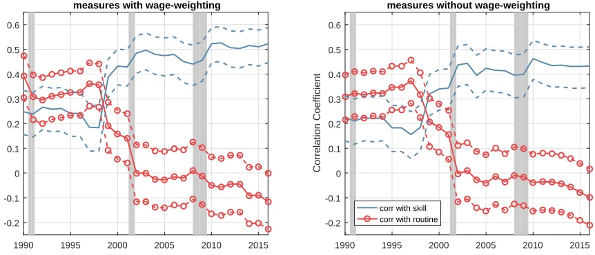
1.12 Correlation of Offshorability with Skill/Routine over time . . . . 91
1.13 Trade Balances in Goods . . . 91
1.14 Responses of Current Accounts . . . 109
2.1 Smoothed Fiscal Uncertainty . . . 144
2.2 Autocorrelation Functions . . . 145
2.3 Impulse Responses to Structural Shocks . . . 146
2.4 Impulse Responses to Structural Shocks . . . 147
2.5 IRFs to Government Spending Shock . . . 148
2.6 IRFs to Capital Income Tax Shock . . . 149
2.7 Counterfactual Analysis . . . 150
2.8 IRFs to Government Spending Shock at ZLB . . . 151
2.9 IRFs to Capital Income Tax Shock at ZLB . . . 152
2.10 Government Spending and the Business Cycle. . . 163
3.1 State-dependent (leverage) IR to an uncertainty shock: . . . 206
3.2 State-dependent (dividend-price) IR to an uncertainty shock: . . 207
3.3 The Role of the interaction between Uncertainty and Risk aver-sion in Output: . . . 208
3.4 The Role of the interaction between Uncertainty and Risk aver-sion in Investment: . . . 209
3.5 Impulse Response Function to Preference Shock– Basu and Bundick (2017): . . . 210
3.6 Impulse Response Functions – FGRU (2011) . . . 211
3.7 Impulse Response Function to a Volatility Shock Interest Rates – FGRU (2011) vs BP (2014). . . 212
3.8 Impulse Response Function to Country Spread Level Shock for different values of the holding cost of debt – FGRU (2011). . . . 213
3.9 Impulse Response Function to Technology Shock – Basu and
Bundick (2017) . . . 214 3.10 IR to a uncertainty shock: . . . 220 3.11 Impulse Responses to a Volatility Shock in Interest Rates –
FGRU (2011): . . . 222 3.12 Impulse Responses to a Volatility Shock Interest Rates – FGRU
1.1 Occupation Tasks that define Offshorability . . . 55
1.2 Most Offshorable and Non-Offshorable Manufacturing Industries 56 1.3 Most Offshorable and Non-Offshorable Services Industries . . . . 58
1.4 Correlations . . . 60
1.5 All Industries: Univariate Sorts and Four- and Five-Factor Models 61 1.6 Manufacturing vs Services Industries. . . 63
1.7 Manufacturing - Four- and Five-Factor Models . . . 65
1.8 Subsample Analysis . . . 67
1.9 Panel OLS Regressions - Annual Regressions . . . 68
1.10 Offshorability and Low Wage Countries’ Import Penetration . . 70
1.11 Offshorability and Shipping Costs . . . 71
1.12 Offshorability and Multinational Companies . . . 72
1.13 Model Parameters . . . 73
1.14 Model Simulations: Targeted and Model-Implied Moments . . . 74
1.15 Variance Decomposition, Model Predictions and Counterfactuals 75 1.16 Double-Sorts: Offshorability and U.S. Trade Elasticities . . . 77
1.17 Model Prediction: Consumption CAPM. . . 78
1.18 Occupation Tasks that define Offshorability . . . 93
1.19 Most Offshorable and Non-Offshorable Industries. . . 94
1.20 CAPM and Three-Factor Model . . . 95
1.21 Manufacturing vs. Services: Fama & French Three-Factor Model 96 1.22 Subsample Analysis - Fixed Quintiles . . . 97
1.23 Robustness: Industry Specification . . . 98
1.24 Double-Sorts: Offshorability and China’s Import Penetration . . 99
1.25 Manufacturing - Offshorability and SC Betas . . . 100
1.26 Manufacturing - Offshorability and FX Betas . . . 101
1.27 Low-wage Countries. . . 102
1.28 Model Simulation Results with International Bond Trading . . . 110
2.1 Bond yields and Fiscal Policy: . . . 153
2.2 Bond returns and Fiscal Policy: . . . 154
2.3 Calibrated and Estimated Parameters: . . . 155
2.4 Empirical and Model-Based Unconditional Moments: . . . 156
2.5 Real term structure of interest rates: . . . 157
2.6 Variance Decomposition - The Effect of Structural Shocks: . . . . 158
2.7 Bond returns and Fiscal Policy: . . . 159
2.8 Quarterly time-series regression for bond returns . . . 161
3.1 Variance Decomposition Basu and Bundick (2017) - The Effect of Structural Shocks when the Discount rate shocks have a time-varying second moment . . . 203 3.2 IRF Analysis - The Effect of a Volatility Shocks in FGRU (2011)203 3.3 Variance Decomposition FGRU (2011) - The Effect of Structural
Shocks . . . 204 3.4 Variance Decomposition BP (2014) - The Effect of Structural
Shocks . . . 204 3.5 Variance Decomposition FGRU (2011) when innovations to the
country spread and its volatility are correlated . . . 205 3.6 Variance Decomposition Basu and Bundick (2017) - The Effect
of Structural Shocks when the Technology shocks have a time-varying second moment . . . 205 3.7 Parameters for BB (2017) and BB SV Productivity model
From Local to Global: Offshoring
and Asset Prices
Lorenzo Bretscher1
1.1
Introduction
“The typical ‘Made in’ labels in manufactured goods have become archaic symbols of an old era. These days, most goods are ‘Made in the World’.” Antras (2015)
Over the recent decades, the world economy has seen a gradual dispersion of the pro-duction process across borders. Firms increasingly organize their propro-duction on a global scale and choose to offshore parts, components, or services to producers in foreign coun-tries. The revolution in information and communication technology (ICT) and the dis-mantling of trade barriers allow firms to engage in global production networks, or global sourcing strategies, in order to cut costs.2 For this reason, the choice of production
1I would like to thank Veronica Rappoport, Andrea Vedolin, Ulf Axelson, Oliver Boguth (discussant),
Harris Dellas, Boyan Jovanovic, Ian Martin, Gianmarco Ottaviano, Christopher Polk, Andreas Rapp (discussant), Alireza Tahbaz-Salehi, Andrea Tamoni, Branko Urosevic, Philip Valta, Alexandre Ziegler (discussant) and, especially, Christian Julliard and Lukas Schmid as well as the seminar participants at LSE, the University of Bern, the University of Warwick, Oxford University, Nova School of Business & Economics, CEMFI, INSEAD, HEC Paris, Boston College, Carnegie Mellon University, the University of Chicago, Imperial College, London Business School, the Swiss Economists Abroad Conference, the Belgrade Young Economist Conference, the Doctoral Tutorial of the European Finance Association and the HEC Paris Finance PhD Workshop for valuable comments. I also thank J. Bradford Jensen for sharing his data on industry tradability. All remaining errors are my own.
2In addition to the ICT revolution and lower trade barriers, political developments have led to an
increase in the fraction of world population that actively participates in the process of globalization (Antras (2015)).
location is a potentially valuable decision tool at the firm level. However, firms/indus-tries differ in their ability to engage in offshoring due to the nature of their products and tasks involved in the production process. In short, in the era of globalization, the possibility to take a business from local to global has heterogenous implications for the cross-section of industries.
In this paper, I exploit cross-sectional heterogeneity in the ability to offshore to study how the possibility to relocate the production process affects industries’ cost of capital. In particular, I focus on industries’ ability to offshore the employed labor force and examine whether this is reflected in the cross-section of returns.3 To this end, I construct
a measure of labor offshorability at the industry level. The measure is calculated in two steps. In the first step, using data from the O*NET program of the U.S. Department of Labor, I calculate an offshorability score at the occupation level, as in Acemoglu and Autor (2011).4 In the second step, I aggregate occupation offshorability scores by industry, weighting them by the product of employment and the wage bill associated with each occupation. The resulting data set covers an average of 331 industries per year during the period 1990 to 2016.5
I sort industries in five offshorability quintiles and find that the strategy that is long the low and short the high offshorability quintile portfolios, L-H, yields average annual excess returns of 7.31 percent and a Sharpe ratio of 0.48. This premium is not spanned by well-known risk factors such as Fama and French (2015) and Carhart (1997). Even after controlling for the five factors of Fama and French (2015), L-H generates positive average annual excess returns of 4.18 percent.
Furthermore, I split the sample into manufacturing and service industries. In univari-ate sorts, the L-H excess return spread in manufacturing is two to three times larger in magnitude compared to services. Moreover, for service industries, the premium is explained by the CAPM and a positive loading on the market. For manufacturing in-dustries, on the other hand, common linear factor models fail to explain the returns generated by L-H. Consistent with this, in annual panel regressions at the firm level, I find that lagged industry offshorability significantly predicts annual excess returns for manufacturing but not for service industries. The results for manufacturing firms are
3In a related paper, Donangelo (2014) shows that industries that employ many workers with
trans-ferable skills are more exposed to aggregate shocks.
4A strand of literature in labor economics studies offshoring of tasks at the occupation level. See, for
example, Jensen and Kletzer (2010), Goos and Manning (2007), Goos, Manning, and Salomons (2010), Acemoglu and Autor (2011), and Firpo, Fortin, and Lemieux (2013).
5Industries are defined at the three-digit Standard Industry Classification (SIC) from 1990 to 2001
economically meaningful: a one standard deviation increase in offshorability is asso-ciated with 4% to 5% lower annual excess stock returns. These results are robust to controlling for firm characteristics known to predict excess returns.
A first-order question is what drives the heterogeneity between manufacturing and ser-vices. A potential explanation is based on the degree of foreign import competition. While manufacturing industries have seen a sharp increase in foreign competition, mainly from low-wage countries, this is not the case for service industries.6 I relate my results
to foreign import competition in manufacturing industries using conditional double sorts of excess returns on proxies of import competition and offshorability. I find that the L-H premium is monotonically increasing in import competition.7 The results are robust to different proxies of import competition: First, I use a direct measure of import pene-tration from low-wage countries defined as the imports from low-wage countries divided by the sum of domestic production and net exports in a given industry (see Bernard, Jensen, and Schott (2006a)). Second, I use industry-specific shipping costs as a proxy for barriers to trade.8 These results are consistent with the U.S. having a comparative advantage in providing services but not in manufacturing (see also Jensen (2011)).9
In a related paper, Barrot, Loualiche, and Sauvagnat (2017) focus on manufacturing industries and document that industries more exposed to foreign competition have higher excess returns. While their work establishes that import competition poses risks for an industry, my findings document that offshoring allows industries to hedge these risks. Intuitively, being able to offshore allows firms to fight import competition from low-wage countries by reducing costs through relocating production. Consistent with this argument, a recent paper by Magyari (2017) shows that offshoring enables U.S. firms to reduce costs and outperform peers that cannot offshore.
To further improve understanding of the mechanism, I embed the option to offshore in a two-country general equilibrium dynamic trade model similar to Ghironi and Melitz (2005) and Barrot, Loualiche, and Sauvagnat (2017) with multiple industries and ag-gregate risk. I will refer to the two countries as East and West. My model departs from previous work by allowing firms to offshore part of the production, as in Antras
6This can be seen from U.S. trade balances. While the trade balance in goods is negative and has
decreased sharply over the last 25 years, the trade balance for services is positive and has been stable over time.
7In line with this, many recent empirical studies, such as Autor, Dorn, and Hanson (2013, 2016) and
Pierce and Schott (2016), stress the importance of imports from low-wage countries for understanding the dynamics in U.S. manufacturing industries.
8Shipping costs are calculated as the markup of the Cost-Insurance-Freight value over the
Free-on-Board value, as in Bernard, Jensen, and Schott (2006b).
9The principle of comparative advantage was first elaborated by Ricardo (1821) and formalized by
and Helpman (2004). Moreover, I assume that the East has a comparative cost advan-tage over the West in performing offshorable labor tasks. As a result, offshoring to the East allows Western firms to reduce production costs and diversify aggregate risks. In addition, firms in both countries can export and sell their products abroad.
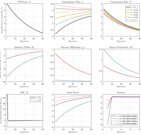
The model successfully matches industry- and trade-related moments and generates return patterns qualitatively, in line with the data. First, it generates a return spread between low and high offshorability industries. Second, the spread is increasing in the degree of import penetration. Third, excess returns of multinational companies are higher than for domestic firms. Fourth, industry excess returns are increasing in import penetration.
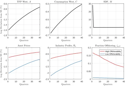
Asset price movements in the model are governed by shocks to aggregate productivity in each of the two countries. The responses of equilibrium quantities to the two ag-gregate productivity shocks are related because quantities react to changes in the ratio of aggregate productivity of the two countries: upon arrival of a positive (negative) productivity shock in the East (West), more Eastern firms find it profitable to export, which results in an increase in import penetration and competition in the West. As a result, Western firms experience losses in market share and lower profits. At the same time, offshoring allows Western firms to reduce production costs, which renders them more competitive towards new market entrants. Consequently, industries with a higher offshoring potential have smoother profits and dividends. Put differently, high (low) offshorability industries are less (more) exposed to aggregate productivity shocks in the model. This difference in exposure to aggregate risk results in an L-H return spread in industry excess returns, as observed in the data.
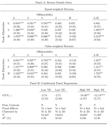
To further validate the model, I test three of its main predictions in the data. First, the model predicts that profit volatility is decreasing in industry offshorability, which is strongly supported by the data: a one standard deviation increase in industry off-shorability is associated with an up to 19.7% lower profit volatility for the median firm. Second, the model predicts that the offshorability premium is largest in industries with more price-sensitive consumers. Conditional double sorts of monthly excess returns on U.S. trade elasticities from Broda and Weinstein (2006) and offshorability confirm this prediction in the data: the L-H spread is roughly double in magnitude for industries with high compared to low U.S. trade elasticities. Finally, within the model, low (high) offshorability industries have high (low) covariance with consumption. Consistent with this, I find that the strategy that is long low and short high offshorability industries has a positive and significant consumption beta in the data.
industry with no offshorability exhibits substantially higher risk premia (up to 33% or 3.14 percentage points) and lower equity valuations (a reduction of up to 17%). Hence, offshoring is an economically important channel in the model.
Finally, within the context of my model, I examine the consequences of a sudden in-crease in trade costs on goods shipped from East to West. Alternatively, this could be interpreted as a sudden increase in trade barriers for all goods imported by the West. Intuitively, higher barriers to trade lead to a decrease in import penetration in the model, which reduces industry risk. However, an increase in trade barriers also renders offshoring less valuable, since shipment of intermediate goods becomes more costly. In-terestingly, within the model, the loss in benefits from offshoring outweighs the positive effects from lower import penetration. As a result, consumption and asset prices in the West fall.
The rest of the paper is organized as follows. After the literature review, section 1.2 details the data and discusses the construction of the labor offshorability measure. In section 1.3, I discuss the empirical findings. Section 1.4 presents a theoretical model with a calibration. Finally, section 1.5 concludes.
Literature Review
This paper relates to four main strands of literature. First, the paper relates to the lit-erature that studies the interaction between labor and asset prices. Danthine and Don-aldson (2002) and Favilukis and Lin (2016) document that operating leverage induced by rigid wages is a quantitatively important channel in matching financial moments in general equilibrium models.10 More recently, a growing body of papers focus on
differ-ent forms of labor heterogeneity and the cross-section of stock returns.11 In particular, Zhang (2016) finds a real option channel for firms that have the possibility to substitute routine-task labor with machines. Moreover, Donangelo (2014) shows that industries with mobile workers are more exposed to aggregate shocks, since mobile workers can walk away for outside options in bad times, making it difficult for capital owners to shift risk to workers. This paper contributes to the literature by studying a new dimension of labor heterogeneity, i.e., whether or not a task can be offshored.
Second, this study relates to the literature on the effects of competition and international trade for asset pricing. Among others Loualiche (2015), Corhay, Kung, and Schmid
10Gomes, Jermann, and Schmid (2017) investigate the rigidity of nominal debt, which creates
long-term leverage that works in a similar way to operating leverage induced by labor.
11See, among others, Gourio (2007), Ochoa (2013), Eisfeldt and Papanikolaou (2013), Belo, Lin, Li,
(2017) and Bustamante and Donangelo (2016) show that the risk of entry is priced in the cross-section of expected returns. In a recent and closely related paper, Barrot, Loualiche, and Sauvagnat (2017) focus on risks associated with import competition and find that firms more exposed to import competition command a sizeable positive risk premium. Furthermore, Fillat and Garetto (2015) document that multinational firms exhibit higher excess returns than purely domestic firms. This is rationalized in a model in which selling abroad is a source of risk exposure to firms: following a negative shock, multinationals are reluctant to exit the foreign market because they would forgo the sunk cost they paid to enter. While their model shows how firms’ revenues relate to risk in multinationals, my paper focuses on the relation between firm risk and labor costs.
Third, a recent line of research studies the consequences of the surge in international trade over the last decades at the establishment and firm level. Among others, Autor, Dorn, and Hanson (2013) and Pierce and Schott (2016) show that U.S. manufacturing establishments more exposed to growing imports from China in their output markets exhibit a sharper decline in employment relative to the less exposed ones.12 Other stud-ies use tariff cuts to instrument for import competition and find that it affects firms’ capital structure (Xu (2012) and Valta (2012)) and capital budgeting decisions (Bloom, Draca, and Van Reenen (2015) and Fr´esard and Valta (2016)). My paper complements this literature by studying asset pricing implications instead of firm quantities. I find that offshoring allows firms to allocate resources more efficiently and lowers risks asso-ciated with foreign import competition.13 Therefore, my paper also contributes to the
growing body of empirical trade literature that documents that manufacturing firms have benefited from offshoring. Hummels, Jørgensen, Munch, and Xiang (2016), Chen and Steinwender (2016) and Bloom, Draca, and Van Reenen (2015) document that off-shoring fosters firms’ productivity and innovation activity. Magyari (2017) shows that offshoring enables U.S. firms to reduce their costs. She also finds that firms that are able to offshore actually increase their total firm-level employment both in manufacturing and headquarter service jobs.14
Fourth, this paper relates to the literature that examines the relationship between firm and plant organization and performance. Empirically, Atalay, Horta¸csu, and Syverson (2013) examine the domestic sourcing by U.S. plants, and Ramondo, Rappoport, and Ruhl (2016) study foreign sourcing by U.S. multinational firms. These papers show that firms and plants tend to source a large share of their material inputs from third-party
12See also Autor, Dorn, and Hanson (2016), Acemoglu, Autor, Dorn, Hanson, and Price (2016), Amiti,
Dai, Feenstra, and Romalis (2016).
13Related papers show that firms suffer less from import competition if they have larger cash holdings
(Fr´esard (2010)) or higher R&D expenses (Hombert and Matray (2017)).
14Compared to other related papers, Magyari (2017) focuses on employment at the firm level rather
suppliers. My paper documents how sourcing decisions affect asset prices. Theoret-ically, Antras and Helpman (2004) formulate a model in which firms decide whether to integrate the production of intermediate inputs or outsource them with incomplete contracts. Both decision can either take place domestically or abroad. More recently, Antras, Fort, and Tintelnot (2016) develop a quantifiable multi-country sourcing model in which global sourcing decisions interact through the firm’s cost function, and Bernard, Jensen, Redding, and Schott (2016) present a theoretical framework that allows firms to decide simultaneously on the set of production locations, export markets, input sources, products to export, and inputs to import. In contrast, my model focuses on the inter-action of offshoring and industry risk. To do so, I incorporate the possibility to offshore into a dynamic trade model with multiple industries, as in Ghironi and Melitz (2005), Chaney (2008) and Barrot, Loualiche, and Sauvagnat (2017).15
1.2
Data
In this section, I first outline the data and the method to construct a measure of labor offshorability at the occupation level and the industry level. Second, I discuss the financial and accounting as well as international trade data used in the empirical analysis.
1.2.1 Measuring Labor Offshorability
As a first step, I calculate a measure of offshorability at the occupation level. To do so, I follow the recent literature in labor economics and use data from the U.S. Department of Labor’s O*NET program on the task content of occupations.16, 17This program classifies occupations according to the Standard Occupational Classification (SOC) system and has information on 772 different occupations.18 O*NET contains information about the tools and technology, knowledge, skills, work values, education, experience and training needed for a given occupation.19 I follow Acemoglu and Autor (2011) and Blinder (2009)
and calculate an offshorability score at the occupation level.
15Melitz (2003) and Bernard, Jensen, Eaton, and Kortum (2003) also allow for firm heterogeneity and
heterogenous gains from trade.
16For papers that rely on the O*NET data base, see, among others, Jensen and Kletzer (2010), Goos
and Manning (2007), Goos, Manning, and Salomons (2010), Firpo, Fortin, and Lemieux (2013), and Acemoglu and Autor (2011).
17I use O*NET 20.3, available fromhttps://www.onetonline.org/
18Some of the 772 occupations are further detailed into narrower occupation definitions. The total
number of more-detailed occupations in O*NET is 954.
19The O*NET content model organizes these data into six broad categories: worker characteristics,
Acemoglu and Autor (2011) argue that an occupation that requires substantial face-to-face interaction and needs to be carried out on site is unlikely to be offshored. To capture this notion of offshorability, they focus on seven individual occupational characteristics, which are tabulated in Panel A of table 1.18. Compared with alternative occupation offshorability scores (see Firpo, Fortin, and Lemieux (2013), for example), Acemoglu and Autor (2011) base their calculations on fewer occupation characteristics to mitigate a high correlation with the routine-task content of an occupation.20
[Insert Table 1.18 here.]
The O*NET database organizes characteristics in work activities or work context (see column 3 of Panel A in table 1.18). For work activities, O*NET provides information on “importance” and “level”. I follow Blinder (2009) and assign a Cobb-Douglas weight of two-thirds to “importance” and one-third to “level” to calculate a weighted sum for work activities.21 Since there is no “importance” score for work context characteristics, I simply multiply the relative frequency by the level.22 Thus, the offshorability score for
occupation j,of fj, is defined as
of fj =
1
PA
l=1I
2 3 jl×L
1 3 jl+
PC
m=1Fjm×Ljm
(1.1)
whereA is the number of work activities, Ijl is the importance and Ljl is the level of a
given work activity in occupation j, C is the number of work context elements, Fjm is
the frequency andLjm is the level of a given work context in occupationj.23 Finally, I
take the inverse to obtain a score that is increasing in an occupation’s offshorability.24
In a second step, I aggregate the occupation offshorability scores at the industry level us-ing industry-level occupation data from the Occupational Employment Statistics (OES) program of the BLS. This data set contains information on the number of employees in a given occupation, industry and year. The data set is based on surveys that track employment across occupations and industries in approximately 200,000 establishments
20As a robustness check, I also calculate occupation offshorability according to Firpo, Fortin, and
Lemieux (2013). They base their calculations on 16 different occupation characteristics, which are organized into three categories: face-to-face contact, on-site and decision-making. The characteristics are tabulated in an online appendix. The results of the paper remain qualitatively the same when the measure of Firpo, Fortin, and Lemieux (2013) is employed and are available upon request.
21The results are robust to different Cobb-Douglas weights. For example, taking simple averages
between importance and level scores does not change any of the results in the paper.
22For example, the level of the work context element “frequency of decision-making” is a number
between one and five: 1 = never; 2 = once a year or more but not every month; 3 = once a month or more but not every week; 4 = once a week or more but not every day; or 5 = every day.
23Note that importance and level scores are all rescaled to be between zero and one. Relative
frequen-ciesFjmlie, by definition, between zero and one.
every six months over three-year cycles, representing roughly 62% of non-farm employ-ment in the U.S. Each industry in the sample was surveyed every three years until 1995 and every year from 1997 onwards. For the period before 1997, I follow Donangelo (2014) and use the same industry data for three consecutive years to ensure continuous coverage of the full set of industries. For example, the data used in 1992 combine sur-vey information from 1990, 1991, and 1992. Unfortunately, the OES did not conduct a survey in 1996. To avoid a gap, I follow Ochoa (2013) and Donangelo (2014) and rely on survey information from the years 1993, 1994, and 1995.
The data set employs the OES taxonomy with 258 broad occupation definitions before 1999, the 2000 Standard Occupational Classification (SOC) system with 444 broad occu-pations between 1999 and 2009, and the 2010 SOC afterwards. To merge the occupation level offshorability with the OES data set, I bridge different occupational codes using the crosswalk provided by the National Crosswalk Service Center. Industries are classified using three-digit Standard Industrial Classification (SIC) codes until 2001 and four-digit North American Industry Classification System (NAICS) codes thereafter.25
The OES/BLS data set also includes estimates of wages since 1997. For the 1990 to 1996 period, I use estimates of wages from the BLS/U.S. Census Current Population Survey (CPS) obtained from the Integrated Public Use Microdata Series of the Min-nesota Population Center.26 I aggregate the occupation level offshorability measure, of fj, by industry, weighting by the wage expense associated with each occupation:
OF Fi,t =
X
j
of fj×
empi,j,t×wagei,j,t
P
jempi,j,t×wagei,j,t
(1.2)
where empi,j,t is the employment in industry i, occupation j and year t, and wagei,j,t
measures the annual wage paid to workers. Using wages at this stage is consistent with placing more weight on occupations with greater impact on cash flows.27 Lastly,OF F
i,t
is standardized in each year, i.e., the cross-sectional mean and standard deviation of the offshorability measure are set to zero and one, respectively. The resulting data set covers the years 1990 to 2016, with an average of 331 industries.
25While the OES data set is designed to create detailed cross-sectional employment and wage estimates
for the U.S. by industry, because of changes in the occupational classification, it might be challenging to exploit its time series variation. For this reason, I focus predominantly on cross-sectional analyses of the data.
26These data are available from https://www.ipums.org/. For more information, see King, Ruggles,
Alexander, Flood, Genadek, Schroeder, Trampe, and Vick (2010)
27I also test for robustness of the empirical analysis by using an industry measure of offshorability
that does not rely on wages, i.e.,
OF Fi,t⋆ =
X
j
of fj× empi,j,t
P
jempi,j,t
.
1.2.2 Financial and Accounting Data
For the empirical analysis, I use monthly stock returns from the Center for Research in Security Prices (CRSP) and annual accounting information from the CRSP/COM-PUSAT Merged Annual Industrial Files. The sample of firms includes all NYSE-, AMEX-, and NASDAQ-listed securities that are identified by CRSP as ordinary com-mon shares (with share codes 10 and 11) for the period between January 1990 and December 2016. I follow the literature and exclude regulated (SIC codes between 4900 and 4999) and financial (SIC codes between 6000 and 6999) firms from the sample. I also exclude observations with negative or missing sales, book assets and observations with missing industry classification codes. Firm-level accounting variables are winsorized at the 1% level in every sample year to reduce the influence of possible outliers. All nomi-nal variables are expressed in year-2009 USD.28 I also use historical segment data from COMPUSTAT to classify firms in multinationals and domestic firms as in Fillat and Garetto (2015). Finally, I use COMPUSTAT quarterly to calculate the volatility of sales and profits, as in Minton and Schrand (1999). A detailed overview of the variable definitions can be found in the online appendix.
1.2.3 International Trade Data
I use product-level U.S. import and export data for the period 1989 to 2015 from Peter Schott’s website. For every year, I obtain the value of imports as well as a proxy for shipping costs at the product level that can be aggregated to the industry level. I follow Hummels (2007) and approximate shipping costs with freight costs, i.e., the markup of the Cost-Insurance Freight value over Free-on-Board value. Moreover, I use data on US trade elasticities at the product level from Broda and Weinstein (2006). Finally, data on U.S. trade balances are from the Bureau of Economic Analysis.
1.3
Empirical Evidence
In this section, I present the empirical results of the paper. First, I examine the validity of the offshorability measures. Second, I report that average portfolio excess returns are decreasing in offshorability. Third, I show that the premium that can be earned by going long low and short high offhsorability industries is concentrated in manufacturing industries and is not explained by a wide range of linear asset pricing models. Finally, I
28I use the GDP deflator (NIPA table 1.1.9, line 1) and the price index for non-residential private
offer further empirical evidence that links the offshorability premium to the recent surge in foreign import competition from low-wage countries.
1.3.1 Validity and Summary Statistics of Labor Offshorability
I start by examining whether the measures discussed in section 1.2 deliver reasonable rankings of occupations and industries in terms of offshorability. Panels B and C of table 1.18 report the top and bottom ten occupations by offshorability. Occupations with high offshorability are not restricted with respect to location or immediacy to the final consumer. Conversely, occupations at the bottom are either closely related to the location, such as “tree trimming”, or to customers, such as “dentists”. Unfortunately, of fj is, by construction, constant throughout time. Therefore, occupation offshorability
is unable to capture how technological progress has affected the offshorability of individ-ual occupations.29To the extent that technological progress has affected offshorability symmetrically across occupations, this is not a concern for my cross-sectional analysis.
In contrast, industry offshorability inherits some time variation from the changes in the occupation-industry composition of the U.S. labor force. To gain a better sense of the time-variation in OF Fi,t, I examine the industry rankings for manufacturing and
services industries separately.30 Table 1.2 reports the top and bottom ten industries by offshoring potential in the years 1992 and 2015 (Panels A and B) and the transition probabilities (Panel C) between offshorability quintiles for manufacturing industries.31 In 1992, the top industries are predominantly apparel industries, whereas the bottom industries are related to mining and construction. The 2015 rankings reveal that there is not much variation over time during the sample period. In fact, even though industries are now classified according to the NAICS system, the top and bottom ten are similar to 1992.32
Another way to examine the persistence of OF Fi,t over time is to look at transition
probabilities. I do so by sorting industries into quintiles of offshorability each year and calculating the transition probabilities across quintiles. Panel C of table 1.2 reports the one- and five-year transition probabilities.33 For industries in the top or bottom
29Several authors note that recent technological advances have substantially increased the
offshorabil-ity of occupations. See, among others, Antras (2015) for manufacturing occupations and Jensen (2011) for service industry occupations.
30Manufacturing industries contain all industries with SIC codes between 2011 and 3999 and NAICS
codes between 311111 and 339999, respectively. Conversely, service industries encompass all industries that are not classified as manufacturing industries.
31An analogous table with industry rankings for the full sample can be found in an online appendix. 32Note that the industries with NAICS code 3341xx correspond to SIC industry 3570, which ranks
18th in 1992.
33I calculate transition probabilities for the period 1991 to 2001 (SIC codes) and 2002 to 2016 (NAICS
quintiles of labor offshorability, the probability of being in the same quintile the next year (in five years) is close to 90% (80%). For the middle quintiles, the persistence is slightly lower, approximately 75%, over one year and 60% over five years. To sum up, industry offshorability is very persistent over time, consistent with offshoring being a slow-moving response to changes in the economic environment.
[Insert Tables 1.2 and 1.3 here.]
Table 1.3 reports analogous industry rankings and transition probabilities for service industries. I find that legal and financial services and computer software programming are high in offshorability, whereas mining, labor unions and other personal services are not.34 Overall, the findings are very much in line with those for manufacturing. Again, the top and bottom ten industries in 1992 and 2015 suggest that OF Fi,t does
not exhibit much variation over time. The transition probabilities in Panel C confirm this impression. The probability of remaining in the same quintile over the next year (next five years) ranges between 83% and 91% (61% and 82%). Moreover, there are only very few changes, other than to the neighboring quintile, even over five years.
Next, I examine how offshorability correlates with other labor- and trade-related vari-ables. Panel A of table 1.4 reports correlations at the occupation level. Interestingly, of fj is positively and significantly related to skill (correlation coefficient of .31), which
is driven by the large number of service occupations that are both offshorable and skill-intense.35 This is in line with Jensen (2011), Blinder (2009) and Amiti and Wei (2009), who discuss that recent advances in communication technologies increasingly allow for the offshoring of service jobs. Importantly, the correlation between offshorability and routine-task occupations is statistically indistinguishable from zero (correlation coeffi-cient of .04). Hence, occupation level offshorability does not solely capture occupations that can be substituted with machines. This is consistent with Zhang (2016), who finds an insignificant empirical correlation coefficient of -.02 between offshorability and routine-task labor at the firm level. In panel B, I report the overlap in occupations that rank in the top tercile for the different measures. I find that the percentage overlap is close to 33%, which is what one would expect in case of no correlation. This suggests that there is little correlation in the highest-ranked occupations across measures.
[Insert Table 1.4 here.]
34Related to this finding, Alan Blinder writes in Foreign Affairs in 2006 that “...changing trade
patterns will keep most personal-service jobs at home while many jobs producing goods and impersonal services migrate to the developing world...”.
35Examples of such occupations include legal support workers or paralegals, computer programmers,
Panel C reports time-series averages of annual Spearman rank sum correlations of differ-ent variables at the industry level both for manufacturing and services. The correlation with skill is positive and significant for both manufacturing and service industries. While the point estimate for manufacturing is very similar to that at the occupation level (.29), it is slightly higher for services (.44). The correlation with routine is statistically indis-tinguishable from zero for both sectors (the point estimates are .10 for manufacturing and .14 for services). Interestingly, the correlation with the labor mobility measure of Donangelo (2014) is negative (-.22) and weakly statistically significant for manufactur-ing and is positive (.11) but insignificant for services. The weak relationship with labor mobility is not surprising. Labor mobility is intended to capture the transferability of occupation-specific skills across industries, which is conceptually very different from offshorability.
Furthermore, I find that the correlation coefficient with product tradability from Jensen (2011) is positive (.13) but insignificant for manufacturing and positive and highly sta-tistically significant for services (.23).36 The insignificant correlation coefficient in man-ufacturing is not surprising. While offshorability captures the “tradability” of the labor force, the measure by Jensen (2011) captures the tradability of the product.
Finally, I also analyze the relation betweenOF Fi,tand industry shipping costs, a variable
often employed in studies of international trade. I document a negative and weakly significant correlation coefficient (-0.16) between offshorability and shipping costs paid by importers for manufacturing industries. For services, the lack of import data makes it impossible to calculate shipping costs at the industry level.
1.3.2 Portfolio Analysis
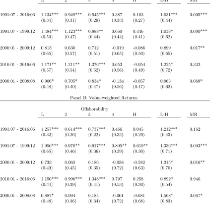
1.3.2.1 Offshorability Portfolios and Excess Returns
To study the characteristics of sample industries and realized excess returns, I construct five offshorability portfolios. For each sample year, I assign industry offshorability in the previous year to individual stocks. I then obtain monthly industry returns by value-weighting monthly stock returns. Again, industries are defined at the 3-digit SIC level between 1990 and 2001 and at the 4-digit NAICS level between 2002 and 2016. In every year, at the end of June, I sort industry returns into five portfolios based on industry offshorability quintiles. Finally, industry returns within each offshorability portfolio are either equal- or value-weighted. To obtain value-weighted portfolio returns, I use an industry’s market capitalization as a weight. In what follows, in the interest of brevity,
36I thank J. Bradford Jensen for sharing his data on industry tradability. Jensen (2011) measures of
I refer to industry excess returns simply as excess returns. Panel A of table 1.5 reports the equal- and value-weighted excess returns of the five portfolios. L (H) stands for the portfolio consisting of industries with low (high) offshorability, and L-H refers to the strategy that is long L and short H.
[Insert Table 1.5 here.]
Industries with low offshorability have average equal-weighted (value-weighted) monthly excess returns that are .61% (.80%) higher compared to high offshorability industries. The magnitude of the spread is economically meaningful: 7.31% (9.64%) per year for equal-weighted (value-weighted) returns with an annualized Sharpe ratio of .48 (.47). I also consider unlevered equity returns to ensure that the results are not driven by leverage. I follow Donangelo (2014) and Zhang (2016) and calculate unlevered stock returns as
runleveredi,y,m =ry,mf + (ri,y,m−rfy,m)×(1−levi,y−1)
where ri,y,m denotes the monthly stock return of firm i over month m of year y, rfy,m
denotes the one-month risk-free rate in month m of year y, and levi,y−1 denotes the
leverage ratio, defined as the book value of debt over the sum of book value of debt plus the market value of equity at the end of year y−1 for firmi. The unlevered excess returns (.51% equal-weighted and .73% value-weighted) and corresponding Sharpe ratios (.46 equal-weighted and .43 value-weighted) are slightly lower in magnitude.
Despite the relatively short sample period, t-tests using Newey-West standard errors confirm that the L-H spread is statistically significant both in equal- and value-weighted portfolios. Notably, the results are slightly stronger for value-weighted returns. While traditional t-tests only compare returns of the L and H portfolios, the “monotonic re-lationship (MR)” test by Patton and Timmermann (2010) tests for monotonicity in returns relying on information from all five portfolios. Next to the L-H spread in table 1.5, I report in parentheses the p-value from the MR test, which considers all possible adjacent pairs of portfolio returns. The bootstrapped p-value is studentized, as ad-vocated by Hansen (2005) and Romano and Wolf (2005). The p-values indicate that the null hypothesis of non-monotonic portfolio returns is rejected both for equal- and value-weighted returns.
(2015).37 Even after controlling for the various factors, the estimated alphas show a nearly (one exception) strictly monotonic pattern for both equal- and value-weighted returns.38 Moreover, the alpha of the L-H portfolio remains statistically significant in three out of four specifications. L-H loads positively on SMB in all specifications. More-over, for equal-weighted portfolios, L-H is positively related to HML. Even though the magnitude of the L-H alpha is smaller than the spread in univariate portfolio sorts, it is economically meaningful: the annualized alphas range between 3.82% and 6.49%, with Sharpe ratios from .35 to .41.
1.3.2.2 Offshorability premium: Manufacturing vs Service Industries
Due to limited data availability, most empirical papers that study the effects of offshoring focus on U.S. manufacturing firms or European data.39 Hence, having a measure of offshorability both for manufacturing and services industries, it is interesting to see how the results differ among these two broad sectors. To this end, I first split the sample into manufacturing and services and then conditionally sort industries into five offshorability portfolios, as discussed above.40
Table 1.6 reports univariate portfolio sorts and CAPM regression results for manufac-turing (Panel A) and services (Panel B). The univariate sorts show that portfolio excess returns are decreasing in offshorability in both sectors, which suggests that the reloca-tion of producreloca-tion is a desirable opreloca-tion in manufacturing and service industries. This is consistent with Jensen and Kletzer (2010), Blinder (2009) and Amiti and Wei (2009), among others, who discuss the increasing importance of offshoring in service industries.
However, the annualized mean excess return of L-H in manufacturing is two to three times the magnitude of that in services: 12.37% versus 6.66% for equal-weighted levered returns and 12.43% versus 4.15% for equal-weighted unlevered returns. This is also true for value-weighted excess returns. Hence, having the option to offshore seems to affect the risk profile of manufacturing and services industries differently. This conclusion finds further support in sector-specific CAPM regression results. For manufacturing, the L-H strategy is not spanned by the market, and the resulting alphas are highly statistically and economically significant. For services, on the other hand, the alphas are insignificant
37The risk-free rate and the market, size, value, momentum, profitability and investment factors are
obtained from Kenneth French’swebsite.
38The results are very similar for the unconditional CAPM, the conditional CAPM and the three-factor
model of Fama and French (1992). The corresponding regressions are tabulated in an online appendix.
39See Harrison and McMillan (2011) and Ebenstein, Harrison, McMillan, and Phillips (2014) for
studies on U.S. data and Hummels, Jørgensen, Munch, and Xiang (2016) for a study with Danish data.
40Manufacturing includes all industries with SIC codes between 2011 and 3999 and NAICS codes
and are only roughly one-third in magnitude compared to manufacturing. In short, while differential exposures to the market across the five offshorability portfolios explain the offshorability spread in services, this is not the case in manufacturing.41
[Insert Tables 1.6 and 1.7 here.]
Panel C of table 1.6 shows portfolio characteristics of the five portfolios in manufacturing and services, respectively. For manufacturing, firms with low offshorability tend to be large, have a low book to market ratio, low market leverage and low labor intensity compared to high offshorability firms. For services, on the other hand, the five portfolios show no clear patterns in terms of book to market ratio and market leverage.
As a more restrictive test of the offshorability premium in manufacturing, I employ the four- and five-factor models by Carhart (1997) and Fama and French (2015), respectively. The results are reported in table 1.7. The alpha of the L-H strategy remains highly statistically and economically significant across all specifications: the annualized alphas range between 8.05% and 9.94% with Sharpe ratios from .55 to .81. Moreover, L-H positively loads on size and momentum.
To gain an idea of the performance of L-H in each sector over time, I plot the evolution of a one USD investment on a log-scale in the left panel figure 1.1. The figure plots L-H separately for manufacturing and service industries along the market, size and value. Both L-H portfolios significantly outperform the size and value strategies over the period from July 1991 until June 2016.
[Insert Table 1.8 and Figure 1.1 here.]
Interestingly, the L-H strategy in manufacturing does not generally correlate strongly with the market except during the financial crisis, when both investments lose value. The right panel of figure 1.1 plots the realized equal-weighted excess returns of the L-H strategy in manufacturing along with average monthly excess returns for the first and second half of the sample period. The two averages are similar in magnitude (1.19% during 1991 and 2004 and 0.86% during 2004 and 2016), which suggests that the L-H strategy delivers a stable return over time.
To further investigate the offshorability premium in manufacturing, I report portfolio sorts for different time subsamples in table 1.8. The sample is split into four subsamples - one for each decade plus one that excludes the financial crisis. The offshorability
41These results also hold for the three-factor model of Fama and French (1992): the L-H for
premium is, with one exception, positive and significant in all subsamples. This is true both for equal- and value-weighted portfolios. For most subsamples, the premium is significant at the 10% level due to the relatively small sample size and the corresponding loss of statistical power. Moreover, the MR-test rejects the null hypothesis of non-monotonic portfolio returns for all but the most recent subsample that runs from 2010:01 to 2016:06.42
In a next step, I investigate the predictive power of offshorability in the cross-section of returns. To do so, I run annual panel regressions at the firm level. The regressions are of the following form:
ri,t=a+bj,t+c∗OF Fi,t−1+d∗controlsi,t−1+ǫi,t, (1.3)
whereri,t is the firm’siannual stock return,ais a constant term,bj,tis an industry×year
fixed effect,OF Fi,t−1 is lagged labor offshorability andcontrolsi,t−1are lagged firm-level
characteristics.43 I include firm size, book-to-market ratio, market leverage ratio, hiring rate, investment rate, one-year lagged stock return, operating leverage, and profitability to control for characteristics known to predict expected excess returns. Standard errors are clustered at the firm and year level.
Table 1.9 reports the regression results for manufacturing in Panel A and services in Panel B. All variables are standardized with mean zero and variance one, which makes the coefficients directly comparable. For manufacturing, the coefficient of offshorability is negative and statistically significant across all specifications. Moreover, the coefficients are only marginally affected by adding control variables individually (compare regression specifications (1) to (9)), which is reassuring.44 The estimated slopes range from -4.64 to -5.06 and are economically meaningful: a one standard deviation increase in offshorability is associated with a 4% - 5% lower annual excess stock return.
[Insert Table 1.9 here.]
Regression specification (10) includes all control variables at once, which results in a reduction in sample size. Nevertheless, the coefficient on OF Ft−1 stays negative and
42In a robustness test, I test whether the results are driven by the time variation in theOF F
i,tmeasure. I find that keeping industry offshorability fixed over time (i.e., fixing it to the first observation for each industry classification period) results in very similar full and subsample results. The corresponding results are tabulated in an online appendix.
43Note that offshorability is measured at the industry level only. Hence, firms in a given industry and
year share the same offshorability.
44I run similar monthly panel regressions following Belo, Lin, Li, and Zhao (2015) and find that the
highly statistically significant.45 For services, the coefficients on offshorability are neg-ative throughout all specifications. However, the coefficients are statistically significant only in two regression specifications, which suggests that for services, OF Ft−1 does
not have much predictive power once controlled for other firm characteristics. This is consistent with the findings of table 1.6.
1.3.3 Manufacturing Industries and the Surge in International Trade
Technological advances such as the revolution in information and communication tech-nologies and the dismantling of trade barriers have contributed to an increase in inter-national trade activity over the recent past. The left panel of figure 1.2 shows that the ratio of imports to U.S. Gross Domestic Product (GDP) has increased by a factor of 1.5 over the sample period. Interestingly, this increase in imports/GDP is mostly due to imports from low-wage countries, which have increased by a factor of 4.5 since 1990. By contrast, high-wage country imports have increased by a factor of 1.2 only.46 These
growth patterns are illustrative of the change in the composition of U.S. imports, con-sistent with the principle of comparative advantage first elaborated by Ricardo (1821) and continued by Heckscher (1919) and Ohlin (1933).47 They argue that countries have a comparative advantage in activities that are intensive in the use of factors that are relatively abundant in the country. As a result, countries that have an abundance of low-cost labor have an advantage in producing labor-intense products, and countries with an abundance of skilled labor specialize in skill-intense products.
[Insert Figure 1.2 here.]
Another way of illustrating the change in the composition of U.S. imports is to look at the trade balances for goods and services separately, as reported in the right panel of figure 1.2. While the trade balance in goods has decreased sharply over the last 25 years, the trade balance in services has been positive and slightly increasing since 1960. Hence, the United States is a net exporter in services.48 Consistent with this, Jensen (2011) argues that providing services is consistent with the U.S.’s comparative advantage. On the other hand, international specialization has led to fierce import competition in manufacturing
45These results are robust to various industry definitions. The corresponding results are tabulated in
an online appendix.
46I follow Bernard, Jensen, and Schott (2006a) and label a country as low-wage in yeartif its GDP
per capita is less than 5% of the GDP per capita of the U.S. A list of countries that were classified as low-wage in every year of the sample period can be found in an online appendix.
47The figure that plots value shares of imports instead of real value of imports looks nearly identical.
The corresponding figure can be found in the online appendix of the paper.
48In fact, the United States is the global leader in business service exports. The OECD reports that
industries.49 In fact, many recent empirical studies stress the importance of international trade for understanding the dynamics in U.S. manufacturing industries. In particular, the rise in import penetration from low-wage countries has been emphasized as the key driving force of the decrease in manufacturing employment (see, among others, Autor, Dorn, and Hanson (2013, 2016), Pierce and Schott (2016)).50
Motivated by this evidence, I examine how my results relate to import competition from low-wage countries. I follow Bernard, Jensen, and Schott (2006a) and calculate import penetration from low-wage countries at the industry level. Panel A of table 1.10 reports conditional double sorts on import penetration and offshorability.51 Indeed, the L-H
spread is monotonically increasing with import penetration both for equal- and value-weighted returns. This finding is consistent with the interpretation that the ability to relocate production is most valuable in industries that are exposed to fierce import competition from low-wage countries.52
[Insert Tables 1.10 and 1.11 here.]
I also run cross-sectional return predictability regressions conditional on import pene-tration being lower (higher) than the median, which allows me to control for various firm characteristics. The results are reported in Panel B. Consistent with the double sorts, I find that coefficients on offshorability are negative and significant only for firms in industries with high import penetration. Moreover, the absolute values of the esti-mated coefficients onOF Ft−1are double the magnitude for high compared to low import
penetration industries.
A potential concern is that realized U.S. imports from low-wage countries may be cor-related with industry import demand shocks. To mitigate this concern, I instrument for import competition with industries’ average shipping costs paid on imports, which serves as a proxy for barriers to trade. In the data, industries with low shipping costs are associated with high imports and exports. Panel A of table 1.11 reports average re-turns of conditional double sorts on shipping costs and offshorability. The L-H spread is monotonically decreasing with shipping costs, consistent with the findings in table 1.10.
49The increase in imports is either due to new market entrants or imports of intermediate production
inputs. Antras (2015) reports that between 2000 and 2011, close to 50% of imports were intra-firm transactions, i.e., either intermediate production inputs or final goods manufactured entirely abroad. The other half of imports were either third-party intermediate goods or final products of foreign competitors. Hence, the surge of imports from low-wage countries over the past 25 years brought cheaper intermediate production inputs but also more fierce competition to the U.S.
50While US total imports as a share of GDP have increased from 4.19% to 15.48% since 1960, US
manufacturing employment as a percent share of nonagricultural employment has fallen from 28.43% to 8.69%. A corresponding figure can be found in the online appendix.
51I first sort on import penetration and then on offshorability.
52The results are very similar for double sorts on offshorability and import penetration from China,
Panel B tabulates the results of conditional panel regressions. Offshorability negatively predicts firms’ annual excess returns only in industries with lower-than-median shipping costs.
Barrot, Loualiche, and Sauvagnat (2017) document that industries with low shipping costs face higher import competition and have higher excess returns. This premium originates from the risk of displacement of least efficient firms triggered by import com-petition. Given that the offshorability premium is increasing in import penetration from low-wage countries and decreasing in shipping costs, my findings suggest that offshoring helps protect industries from foreign competition. In particular, being able to offshore allows firms to reduce their labor costs upon increases in competition. This argument is consistent with Magyari (2017), who finds that offshoring enables US firms to reduce costs and outperform peers that cannot offshore.
Table 1.4 shows that offshorability is slightly negatively related to shipping cost. Hence, one might be concerned whether sorting on offshorability is similar to sorting on ship-ping costs. To mitigate this concern, I replicate the findings of Barrot, Loualiche, and Sauvagnat (2017) for my sample period and control for the return of the portfolio that is long firms in low shipping cost industries and short firms in high shipping cost indus-tries (henceforth, SC). The explanatory power of SC is very limited. In fact, neither the monotonic relationship in the offshorability portfolio alphas nor the highly statistically significant alpha of the L-H portfolio is impaired.53
Approximately half of the manufacturing firms in my sample are multinational compa-nies that have sales in at least one country other than the United States. Fillat and Garetto (2015) have documented that multinational firms experience higher stock re-turns compared to domestic firms. To understand how their results relate to mine, I first split the sample into multinat