MATLAB based modeling to study the effects of partial shading on PV array characteristics

(1)

© 2016, IRJET | Impact Factor value: 4.45 | ISO 9001:2008 Certified Journal

| Page 2180

MATLAB-based modeling to study the effects of partial shading on

PV array characteristics

A.S.L.V.SWATHI

,

Dept. of EEE

GVPCOE (A), Visakhapatnam.

G.VANITHA

Dept. of EEE

GVPCOE (A), Visakhapatnam.

Abstract-- The performance of a photovoltaic (PV) module is mostly affected by array configuration, irradiance, and module temperature. It is important to understand the relationship between these effects and the output power of the PV array.This work presents a MATLAB-Simulink-based PV module model which includes a controlled current source and an Function builder. The modeling scheme in S-Function builder is deduced by some predigest functions. Under the condition of non-uniform irradiance, simulation show that the output power of a PV array gets more complicated due to multiple peaks. Moreover, the proposed model can also simulate electric circuit and its maximum power point tracking (MPPT) in MATLAB-Simulink.

Keywords _MATLAB-Simulink, model, non-uniform irradiance, photovoltaic (PV)

I .INTRODUCTION

With a spurt in the use of renewable energy sources, photovoltaic (PV) power generation is being employed in many applications. Conventionally, a PV system consists of solar PV arrays and electric converters. A PV array is formed by series/parallel combination of solar modules. SomeoperatingconditionsresultinnonuniformirradianceofP Varray,such as shadows, clouds, dirt, debris, bird droppings, different orientations and tilts, and so on. If several solar cells in a series PV module are mismatched due to non uniform irradiance, these cells will limit the output current of normal cells. This leads to decrease of the output power, even generates hot-spot and causes damage to these cells. To avoid the destructive effects of hotspot, a bypass diode is connected in parallel with a PV module or parallel with some series-connected solar cells in a PV module, which creates a replacement path [1]. The output power of mismatched cells is cut off when the bypass diode works. The output characteristics will be more complicated when the PV array is mismatched, and it causes some energy loss [2]–[5]. To obtain maximal PV installation output power, it is very important to reveal PV characteristics under condition of non-uniform irradiance. To model solar cell, the one-diode model has been proposed [6], and some researchers have studied how to extract parameters for the model [7], [8]. For a higher

accuracy, two diode model has been studied for years [9], [10]. In these research works, some methods were developed to determine the electrical parameters in these models. The electrical characteristics of a solar cell/PV module derived from those proposed models match the experimental data well when irradiance is uniform. However, these models cannot be directly used when irradiance is non-uniWith a spurt in the use

(2)

© 2016, IRJET | Impact Factor value: 4.45 | ISO 9001:2008 Certified Journal

| Page 2181

EQUIVALENT CIRCUIT OF SINGLE SOLAR CELL

To achieve a simulation kit of this issue, a simple but accurate enough PV module model using MATLAB-Simulink was proposed in this paper. It is derived from a one-diode model with some parameters in the main formula, which could make calculating easier. The proposed model can not only be combined to simulate PV array by series/paralleled connection, but also be employed to simulate an electronic circuit and its control strategy, especially under conditions of non- uniform irradiance.

Fig.1. Equivalent circuit of a single solar cell

II. PHOTOVOLTAIC MODULE MODELING

A. Mathematical Equation of a Solar Cell

There are many equivalent circuits of a solar cell, where the single-diode and two-diode models could be the most widely used. Since the single-diode model is simple and accurate enough in many cases [7], [8], it is applied in this paper. Its equivalent circuit with series and parallel resistance is shown in Fig. 1 [22].

The symbols in Fig. 1 are deﬁned as follows:

Iph: photocurrent;

Id: current of parallel diode;

Ish: shunt current;

I: output current;

V : output voltage;

D: parallel diode;

Rsh: shunt resistance;

Rs: series resistance.

The I–V equation of Fig. 1 is showed as

I=Iph-Io {e(V+I.Rs/VI)-1}-(V+RsI/Rsh) (1)

Where Io is the reverse saturation current of the diode, q is the electron charge (1.602×10−19 C), A is the curve ﬁtting factor, and K is Boltzmann constant (1.38×10−23J/K).

B. Model of a PV Module

If a solar cell type tends to have an I–V curve in which the slope at short circuit is almost zero, the value of Rsh can be assumed to be inﬁnite [23]. In this case, the last term in (1) could be ignored. And taking Iph as ISC, (1) will become [22]

I = ISC −Io (e (V + R s I ) AKT −1) (2)

where ISC is the short-circuit current.

Equation (2) is valid for a solar cell. For the accurate application of this equation for a PV module, the term of q(V + RsI)/AKT is changed to q(V + RsI)/NsAKT, in which Ns is the number of series-connected solar cells in a PV module. Then, (2) will become

I = ISC −Io (eq (V + R s I )/ N s AKT −1) (3).

Under standard test condition (STC), which consists of a PV module temperature of 25 ◦C and an in-plane irradiance of 1 000 W/m2 with spectral distribution conforming to an AM1.5 spectrum, (7) could be rewritten as follows:

Iref = ISC,ref(1−k V ref+ R s Iref Voc,ref −1)

Where Iref is the output current under STC, ISC,ref is the short circuit current under STC, Vref is the output voltage under STC, VOC,ref is the open-circuit voltage under STC, and kref is the coefficient of k under STC. Parameters at maximum output power point (MPP) under STC could be given to solve the coefficient of kref

kref = ( V MPP,ref+ R s IMPP,ref V OC,ref −1)1− IMPP,ref ISC,ref

(3)

© 2016, IRJET | Impact Factor value: 4.45 | ISO 9001:2008 Certified Journal

| Page 2182

C. PV Module Model in MATLAB-Simulink

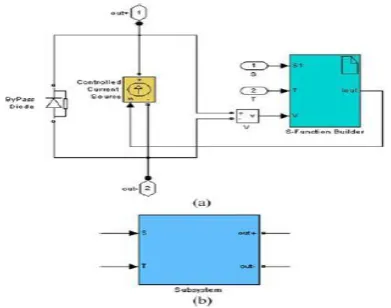
[image:3.595.308.557.146.466.2]

The block diagram of the MATLAB-Simulink-based PV module model is shown in Fig. 3(a), where the proposed model and the ﬂow in sector B are implemented by an S-Function builder with three inputs and one output. S1 is

Fig 2. PV module in MATLAB Simulink

Irradiance, T is the temperature of the PV module, V is the output voltage of the PV module, and I out is the output current of the PV module. I out connecting to a controlled current source is used for sim ulating the output current of the PV module. A bypass diode is connected in parallel with the controlled current source.

For the sake of convenience, all components in Fig. 2(a) are incorporated into a subsystem block in following steps.

Step 1: Enclose the blocks and connect lines in Fig. 2(a) within a bounding box.

Step 2: Choose the option of create subsystem from the Edit menu. MATLAB-Simulink replaces the selected blocks with a subsystem block, which is shown in Fig. 2(b).

The subsystem block in Fig. 2(b) will be a basic PV module mode of MATLAB-Simulink in this paper. In the subsystem block, port of out + is the positive terminal of the PV module, port of out− is the negative terminal of the PV module, port of S is the in-plane irradiance, and T is the temperature of the PV module. The subsystem blocks can be connected in series/parallel according to the actual PV array; then it can be simulated in MATLAB-Simulink.

Fig. 3 shows the details of the screen shot of a S-Function builder block [see Fig. 2(a)]. The pane of port/parameter displays the ports and parameters that the dialog box speciﬁes for the target S-function; they are S1, T1, V , and Iout. All ports are in complexity of real and dimension of

1-D. The S-code for the implementation of the proposed ﬂow in resides in the output pane. The S-code is presented in the Appendix.

Fig 3.Screen shot of S-function builder

III. EXPERIMENTAL VALIDATION OF THE MODEL

This section describes the procedure and results using the proposed MATLAB-Simulink based model. It is important to understand how the model works under different conditions. A PV module, EGing-50W, produced

by EGING PV with

36series-connectedmonocrystallinecells,is chosen to evaluate the proposed model in this paper. The electrical characteristics

[image:3.595.43.239.182.336.2]

(4)

© 2016, IRJET | Impact Factor value: 4.45 | ISO 9001:2008 Certified Journal

| Page 2183

Parameters Variable Value

Maximum

power Pmax 50W

Voltage at

pmax Vmpp 17.98V

Current at

pmax Impp 2.77A

The parameters of series resistance Rs, irradiance correction factor in ,and coefficient kref have to be determined. It is well known that the derivative of the PV module power with respect to the PV module voltage is zero at MPP. An additional equation to obtain an analytical solution for Rs can be achieved [25]. The following formula can be obtained at MPP:

dI dV |V =VMPP =−IMPP VMP.

On the other hand, the derivative of (7) with respect to V brings

dI dV =−ISC

1+Rs dI dV VOC kV + R s I V OC −1 lnk. (16)

Equation (16) could be rewritten at MPP as follows:

[image:4.595.53.293.99.238.2] [image:4.595.345.526.245.386.2]

dI dV |V =VMPP=−ISC

1+Rs dI dV |V =VMPP VOC k

V MPP+ R s IMPP V OC −1lnk. (17)

. Substituting (9) and (15) into (17) under STC, an expression of Rs will be obtained as follows:

Rs = VMPP,ref + IMPP,ref(VOC,ref−VMPP,ref) (ISC,ref−IMPP,ref) ln(1−IMPP,ref ISC,ref)/

(IMPP,ref + I2MPP,ref (ISC,ref−IMPP,ref) ln(1−IMPP,ref ISC,ref) (18)

Rs of a PV module EGing-50W is 0.085 Ω by substituting the parameters in Table I into (18) and the coefﬁcient kref is 3 047 214 by using (9). Rs is assumed to be a constant at its reference value under STC [23].

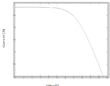
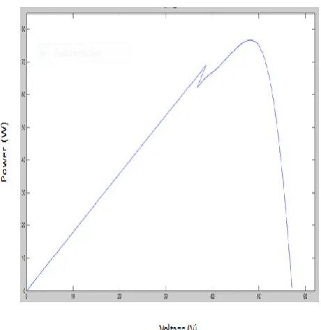
A. Study Case of a Single PV Module

To evaluate the availability of the proposed model, three measurement I–V curves and P–V curves of single EGing-50W PV module under outdoor condition are selected to compare the results of simulation using the proposed model. Testing conditions are irradiance at 890 W/m2with module temperature at 50 ◦C.

Fig 4 Simulation of I- V curve

Fig 5 Simulation of P-V curve

B. Study Case of a PV Array under the Conditions of Non -uniform Irradiance

(5)

© 2016, IRJET | Impact Factor value: 4.45 | ISO 9001:2008 Certified Journal

| Page 2184

are the same due to covering quickly and

[image:5.595.308.560.98.379.2]

measuring immediately.

Fig 6 simulation of IV curve under non uniform irradiance

Fig 7 Simulation of PV curve under non uniform irradiance

Obviously, the numbers of power peaks depend on in-plane irradiance levels in the series of PV modules .Note that the short circuit current of each PV module under different irradiance is different ;the associated bypass diode would be conducted when the passi ng current is greater than its short-circuit current. That means the PV module is cut off and is not able to produce any electricity power. So, different in-plane irradiance levels in the series of PV modules might cause different numbers of power peaks depending on how many PV modules are bypassed. Given a PV array which consists of six PV modules arranged into two parallels, each having three modules connected in series. The corresponding simulation diagram is shown in Fig.8

Fig 8 Simulation of PV module under bypass diode condition

[image:5.595.76.281.142.291.2] [image:5.595.49.295.356.507.2] [image:5.595.306.537.433.671.2]

(6)

© 2016, IRJET | Impact Factor value: 4.45 | ISO 9001:2008 Certified Journal

| Page 2185

Fig 9 Simulation result of IV curve under bypass diode

condition

C. Study Case of a Combining Model With DC/DC Converter

To verify the suitability of the proposed model combining with dc/dc converter, a simulation schematic is presented in Fig.11.It consists of series-connected three PV module models and a boost circuit. The boost circuit is a typical ldc/dc converter, and the parameters are set as follows:

L =1 .7mH; R load = 86 Ω;C = 470μ F; and C1 = 10μF

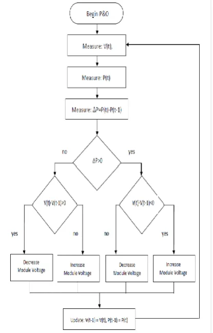
For comparison, the testing platform is configured as the same layout of the simulation schematic in Fig. 14. A same global maximum power point tracking (GMPPT) strategy is applied in both simulation and testing platform. There were some complicated GMPPT strategies [26].For convenience, a simple strategy is adopted; its flow is shown in Fig. 15. Some parameters in the control flow are as follows: initial duty of pulse width modulation is 0.125, V min is 27 V, ΔD is 0.020, duty step in perturb and observe method is 0.020, and control period is 10 ms.

[image:6.595.38.477.60.373.2]

Fig 11.Simulation of boost topology using proposed model

[image:6.595.310.518.378.702.2]

(7)

| Page 2186

RESULTS OF SIMULATION IN THE CASE OF UNIFORM

IRRADIANCE

RESULTS OF SIMULATION IN THE CASE OF NON-UNIFORM IRRADIANCE

IV CONCLUSION

(8)

| Page 2187

condition of non-uniform irradiance. Another important

performance of the proposed model is that a PV array, created by using a proposed model, allows to be combined with an electronic circuit to simulate the behavior of circuit and control strategies. The model is proposed not only to study the behavior of PV array, but also to validate new electronic circuit and MPPT strategies.

APPENDIX

//source code of s-function as follow

Float Isc_ref, Voc_ref, Impp_ref, Vmpp_ref, Rs, Isc, Voc;

Float S ref, T ref;

Float a, b, c;

Float DT;

Double k, I ref, n, V1, D Iref;

Isc_ref=3;

Voc_ref=22; Impp_ref=2.77;

Vmpp_ref=17.98; a=0.0004;

b=-0.0033;

c=0.066; Rs=0.085;

Sref=1000; Tref=25;

DT=T[0]-Tref;

Isc=Isc_ref*(S1[0]/Sref)*(1+a*DT);

Voc=Voc_ref*(1+b*DT+c*log(S1 [0]/Sref));

k=POW (1-Impp_ref/Isc_ref, Voc_ref/ (Vmpp_ref-Voc_ref+Rs*Impp_ref));

Iref=1.5; DIref=1.5;

V1=Voc-Rs*Iref*Isc/Isc_ref+Voc_ref*log (1-Iref/Isc_ref)/log (k);

//Solving (14) in paper via numerical method

For (n=0;n<50;n++)

DIref=DIref/2; if (V1<V[0])

{

Iref=Iref-DIref;

}

elseif (V1>V[0]) {

Iref=Iref+DIref; }

n=100;

}

V1=Voc-Rs*Iref*Isc/Isc_ref+Voc_ref*log

(1-Iref/Isc_ref)/log (k); I out [0]=Iref*Isc/Isc_ref References:

1.H. Patel and V. Agarwal, “MATLAB-based modeling to study the effects of partial shading on PV array characteristics,” IEEE Trans. Energy Convers., vol. 23, no. 1, pp. 302–310, Mar. 2008.

2. ] W. De Soto, S. A. Klein, and W. A. Beckman, “Improvement and validation of a model for photovoltaic array performance,” Solar Energy, vol. 80, no. 1, pp. 78–88, Jan. 2006

3. L. Sandrolini, M. Artioli, and U. Reggiani, “Numerical method for the extractionofphotovoltaicmoduledouble-diodemodelparametersthrough cluster analysis,” Appl. Energy, vol. 87, no. 2, pp. 442–451, 2010.

4. E. V. Paraskevadaki and S. A. Papathanassiou, “Evaluation of MPP voltage and power of mc-Si PV modules in partial shading conditions,” IEEE Trans. Energy Convers., vol. 26, no. 3, pp. 923–932, Sep. 2011.

5. A. K.Sinha, V.Mekala, and S. K. Samantaray,“Design and testing of PV maximum power tracking system with MATLAB simulation,” in Proc. IEEE Region 10 Conf., Nov. 2010, pp. 466–47.