Evolution of the dark matter phase-space density distributions of
CDM
haloes
Ileana M. Vass,
1,2Monica Valluri,
2,3Andrey V. Kravtsov
2,4,5and Stelios Kazantzidis
61Department of Astronomy, University of Florida, Gainesville, FL 32611, USA
2Kavli Institute for Cosmological Physics, The University of Chicago, Chicago, IL 60637, USA
3Department of Astronomy, University of Michigan, Ann Arbor, MI 48109, USA
4Enrico Fermi Institute, The University of Chicago, Chicago, IL 60637, USA
5Department of Astronomy & Astrophysics, The University of Chicago, 5640 S. Ellis Ave., Chicago, IL 60605
6Center for Cosmology and Astro-Particle Physics, The Ohio State University, Columbus, OH 43210, USA
Accepted 2009 February 4. Received 2009 February 2; in original form 2008 October 1
A B S T R A C T
We study the evolution of phase-space density during the hierarchical structure formation of cold dark matter (CDM) haloes. We compute both a spherically averaged surrogate for phase-space density (Q=ρ/σ3) and the coarse-grained distribution functionf(x,v) for dark matter (DM) particles that lie within ∼2 virial radii of four Milky Way sized dark matter haloes. The estimatedf(x,v) spans over four decades at any radius. DM particles that end up within 2 virial radii of a Milky Way sized DM halo atz=0 have an approximately Gaussian distribution in log (f) at early redshifts, but the distribution becomes increasingly skewed at lower redshifts. The valuefpeakcorresponding to the peak of the Gaussian decreases as the
evolution progresses and is well described byfpeak(z)∝(1 +z)4.5 for z >1. The highest
values off (responsible for the skewness of the profile) are found at the centres of dark matter haloes and subhaloes, wheref can be an order of magnitude higher than in the centre of the main halo. We confirm thatQ(r) can be described by a power law with a slope of−1.8±0.1 over 2.5 orders of magnitude in radius and over a wide range of redshifts. ThisQ(r) profile likely reflects the distribution of entropy (K≡σ2/ρ2/3
DM∝r1.2), which dark matter acquires as
it is accreted on to a growing halo. The estimatedf(x,v), on the other hand, exhibits a more complicated behaviour. Although the median coarse-grained phase-space density profileF(r) can be approximated by a power law,∝r−1.6±0.15, in the inner regions of haloes (<0.6r
vir), at
larger radii the profile flattens significantly. This is because phase-space density averaged on small scales is sensitive to the high-f material associated with surviving subhaloes, as well as relatively unmixed material (probably in streams) resulting from disrupted subhaloes, which contribute a sizable fraction of matter at large radii.
Key words: methods: N-body simulations – galaxies: evolution – galaxies: formation –
galaxies: kinematics and dynamics – dark matter.
1 I N T R O D U C T I O N
CosmologicalN-body simulations of the formation of structure in the Universe allow us to reconstruct how gravitationally bound objects like galaxies and clusters form and evolve. These simula-tions have shown that despite the seemingly complex hierarchical formation history of dark matter (DM) haloes, the matter density distributions of cosmological DM haloes are described by simple
E-mail: [email protected]
three-parameter profiles (Navarro, Frenk & White 1996; Merritt et al. 2006).
space occupied by phase-space elements whose density lies be-tween (f,f +df), is also conserved. However, the conservation of the fine-grainedf(x,v) andV(f)dfis not a very useful property for understanding the evolution of real systems, since in practice it is only possible to compute an average offover a finite volume of phase space. This average is referred to as the coarse-grained DF ¯f(x,v), and the associated volume density is ¯V(f). The evo-lution of the coarse-grained DF is governed byMixing Theorems
(Tremaine, Henon & Lynden-Bell 1986; Binney & Tremaine 1987; Mathur 1988). These theorems state that if the coarse-grained DF is bounded, then processes that operate during the relaxation of collisionless systems (e.g. phase mixing, chaotic mixing and the mixing of energy and angular momentum that accompanies violent relaxation) result in a decrease in the coarse-grained phase-space density. This is because at any point in phase space, both low and high phase-space density regions get highly mixed (Tremaine et al. 1986; Binney & Tremaine 1987). In addition, there are simple rela-tionships that exist between the initialV(f) and the coarse-grained
¯
V(f) at a later time: ¯V(f) is always greater thanV(f) (Mathur 1988). Since it is only possible to measure the coarse grained phase-space density, hereafter we simplify the notation and usef(x,v) to represent ¯f(x,v) andV(f) to represent ¯V(f).
Recently, Dehnen (2005) proved a new Mixing Theorem that states that the excess-mass function D(f), which is the mass of material with coarse-grained phase-space density greater than a valuef, always decreases due to mixing, for all values off. He showed, using this theorem, that steeper cusps are less mixed than shallower ones, independent of the details of the DF or density profile, and this implies that a merger remnant cannot have a cusp that is either steeper or shallower than the steepest of its progenitors. Taylor & Navarro (2001) have introduced a surrogate quantity,
Q(r)=ρ(r)/σ(r)3, whereρ(r) is the configuration-space density averaged in spherical shells, andσ(r) is the velocity dispersion of DM particles averaged in a spherical shell centred at the radius
r. Note that, althoughQ(r) has dimensions of phase-space den-sity, it isnottrue coarse-grained phase-space density, because it is constructed out of separately computed configuration-space density and velocity dispersion in arbitrarily chosen spherical shells. Con-sequently, it is not expected to obey anyMixing Theorems(Dehnen & McLaughlin 2005) and is generally difficult to interpret in terms of phase-space density. Nevertheless, it is an intriguing quantity, be-cause Taylor & Navarro (2001) show thatQ(r) is well approximated by a single power law,Q∝r−βwithβ≈1.874 over more than 2.5 orders of magnitude in radius for CDM haloes universally, regard-less of mass and background cosmology (see also Ascasibar et al. 2004; Rasia, Tormen & Moscardini 2004). Recent work, however, indicates thatQ(r) profiles are somewhat sensitive to the amount of substructure and the slope of the power spectrum (Knollmann, Knebe & Hoffman 2008; Wang & White 2008).
While power-lawQ(r) profiles are by no means universal for self-gravitating systems in dynamical equilibrium (Barnes et al. 2006), power-law profiles with exactly the same slope were first shown to arise in simple self-similar spherical gravitational infall mod-els (Bertschinger 1985) pointing to a possible universality in the mechanisms that produce them. Austin et al. (2005) extended the early work of Bertschinger (1985) using semi-analytical extended secondary infall models to follow the evolution of collisionless spherical shells of matter that are initially set to be out of dynamical equilibrium and are allowed to move only radially. They concluded that the power-law behaviour of the final phase-space density pro-file is a robust feature of virialized haloes, which have reached equilibrium via violent relaxation. They used a constrained Jeans
equation analysis to show that this equation has different types of solutions and that it admits a unique periodic solution which gives a power-law density profile with slopeβ=1.9444 [compa-rable to the numerical value ofβ = 1.87 obtained by Taylor & Navarro (2001)].
A recent study (Hoffman et al. 2007), followed the evolution of
Q(r) profiles in cosmological DM haloes in constrained simulations designed to control the merging history of a given halo. These authors showed that, during relatively quiescent phases of halo evolution, the density profile closely follows that of a NFW halo, andQ(r) is always well represented by a power-lawr−βwithβ=1.9 ±0.1. They showed thatQ(r) deviates from power law most strongly during major mergers but recovers the power law form thereafter (this is consistent with our findings using a series of controlled merger simulations; Vass et al. 2009). More recently, Wojtak et al. (2008) demonstrated (using a variant of the FiEstAS code) that the DF ofCDM haloes of mass 1014–1015M
can be separated into energy and angular momentum components. They proposed a phenomenological model for spherical potentials and showed that their model DF was a good match to theN-body DFs and was also able to reproduce the power-law behaviour ofQ(r). Despite the insights obtained in these studies, the origin of the universality of
Q(r) is not yet understood, and the question of how this quantity relates to the true coarse-grained phase-space density has not yet been thoroughly investigated. This motivates our study which is focused on the evolution of both Q(r) and phase-space density evolution using a set of self-consistent cosmological simulations of halo formation.
In the last 4 years, three independent numerical codes to compute the true coarse-grained phase-space density fromN-body simula-tions have been developed (Arad, Dekel & Klypin 2004; Ascasibar & Binney 2005; Sharma & Steinmetz 2006). In the Appendix, we compare results obtained with the codes ‘FiEstAS’ (Ascasibar & Binney 2005) and ‘EnBiD’ (Sharma & Steinmetz 2006) at a range of redshifts. However, we only present results obtained with the ‘EnBiD’ code using a specific kernel. Following the submission of this paper, we became aware of the work of Maciejewski et al. (2009). These authors carried out a similar comparison of various coarse-grained phase-space density estimators forN-body simula-tion cosmological haloes atz=0.
In an accompanying paper (Vass et al. 2009), we present an analysis of phase-space andQ(r) evolution during major mergers between CDM-like spherical haloes. We show that major mergers (those which are the most violent and therefore likely to result in the greatest amount of mixing in phase space) preserve spherically averaged phase-space density profiles [bothQ(r) andF(r)] out to the virial radiusrvir of the final remnant. We confirm the predic-tion (Dehnen 2005) that the phase-space density profiles of DM haloes are extremely robust, and in particular, the prediction that the steepest central cusp always survives.
mergers (such as those studied by Dehnen 2005; Vass et al. 2009) are instructive, they represent the most extreme form of mixing, and are not the major mode of mass accretion in the Universe. In addition, since experiments with major mergers demonstrate that pre-existing power-law profiles are preserved, they shed little light on the formation of the profiles. Our primary goal is to gain a better understanding of the origin of the power-law phase-space density profiles seen in cosmological DM simulations.
In this paper, we investigate the evolution of the coarse-grained phase-space density in the formation and evolution of four Milky Way sized haloes in aCDM cosmology with cosmological pa-rameters: (m, , h, σ8) = (0.3, 0.7, 0.7, 0.9). In Section 2, we summarize the cosmologicalN-body simulations analysed in this study as well as the numerical methods used to obtain coarse-grained phase-space densities. (The Appendix contains a detailed comparison of the two codes FiEstAS and EnBiD. We also present reasons for our choice of EnBiD, withn=10 smoothing kernel). In Section 3, we describe the properties of the spherically averaged quantityQ(r) as well as the the coarse-grained DF for one Milky Way sized DM halo atz=0, as well as the evolution of the phase-space DF of this halo fromz=9 to the present. In Section 4, we also present results for three additional Milky Way sized haloes. In Sec-tion 5, we present an interpretaSec-tion of the power-law profiles seen inQ(r) and discuss the implications of observed coarse-grained DF in a cosmological context. Section 6 summarizes the results of this paper and concludes.
2 N U M E R I C A L M E T H O D S
The simulations analysed in this paper are described in greater detail in the works of Kravtsov, Gnedin & Klypin (2004) and Gnedin & Kravtsov (2006). The simulations were carried out using the adaptive refinement treeN-body code (ART; Kravtsov, Klypin & Khokhlov 1997). The simulation starts with a uniform 2563 grid covering the entire computational box. This grid defines the lowest (zeroth) level of resolution. Higher force resolution is achieved in the regions corresponding to collapsing structures by recursive refining of all such regions by using an adaptive refinement algorithm. Each cell can be refined or de-refined individually. The cells are refined if the particle mass contained within them exceeds a certain specified value. The grid is thus refined to follow the collapsing objects in a quasi-Lagrangian fashion.
Three of the galactic DM haloes were simulated in a comoving box of 25h−1 Mpc (hereafterL25); they were selected to reside in a well-defined filament atz= 0. Two haloes are neighbours, located 425h−1kpc from each other. The third halo is isolated and is located two Mpc away from the pair. Hereafter, we refer to the isolated halo asG1and the haloes in the pair asG2andG3. Although we analysed all three haloes at the same level of detail we present detailed results forG1. The virial masses and virial radii for the haloes studied are given in table 1 in Kravtsov et al. (2004). The virial radius (and the corresponding virial mass) was chosen as the radius encompassing a mean density of∼200 times the mean density of the Universe. The masses of the DM haloes are well within the range of possibilities allowed by models for the halo of the Milky Way galaxy (Klypin, Zhao & Somerville 2002). The sim-ulations followed a Lagrangian region corresponding to the sphere of radius equal to 2 virial radii around each halo atz=0. This region was resampled with the highest resolution particles of massmp = 1.2×10⁶h−1M
, corresponding to 10243particles in the box, at the initial redshift of the simulation (zi=50). The maximum of 10 refinement levels were reached in the simulations corresponding to
the peak formal spatial resolution of 152h−1parsec. Each host halo is resolved with∼106particles within its virial radius atz=0.
The fourth halo was simulated in a comoving box of 20h−1Mpc box (hereafterL20), and it was used to follow the Lagrangian region of approximately five virial radii around the Milky Way sized halo with high resolution. In the high-resolution region, the mass of the DM particles is mp = 6.1×10⁵h−1M, corresponding to effective 10243 particles in the box, at the initial redshift of the simulation (zi = 70). As in the other simulation, this run starts with a uniform 2563 grid covering the entire computational box. Higher force resolution is achieved in the regions corresponding to collapsing structures by recursive refining of all such regions using an adaptive refinement algorithm. Only regions containing highest resolution particles were adaptively refined. The maximum of nine refinement levels were reached in the simulation corresponding to the peak formal spatial resolution of 150h−1comoving parsec. The Milky Way sized host halo has the virial mass of 1.4×10¹²h−1M
(or 2.3 million particles within the virial radius) and virial radius of 230h−1kpc atz=0.
The peak spatial resolution of the simulations determines the minimum radius to which we can trust the density and velocity profiles. In the following analysis, we only consider profiles at radii at least eight times larger than the peak resolution of the simulations [i.e.≈0.5–0.6h−1comoving kpc orr≈0.004r
vir(z=0)].
2.1 Phase-space density estimators
In this paper, we will focus on the time evolution of the spherically averaged phase-space densityQ(r) as well as the coarse-grained phase-space DFf(x, v) during the formation of the Milky Way sized DM haloes in CDM cosmological simulations described above.
In the last four years, three independent numerical codes to com-pute the coarse-grained phase-space density fromN-body simula-tions have been developed (Arad et al. 2004; Ascasibar & Binney 2005; Sharma & Steinmetz 2006).1These techniques differ in the scheme used to tesselate six-dimensional phase space as well as in the density estimators they use. The first study of coarse-grained DF (Arad et al. 2004) showed that it has its highest values at the centres of DM haloes and subhaloes. They also showed that the volume density of phase-spaceV(f) within individual cosmologi-cal DM haloes atz=0 has a power-law profile over nearly four orders of magnitude inf. The main criticism of this code is that it is not metric-free. The FiEstAS algorithm of Ascasibar & Binney (2005) and the EnBid algorithm of Sharma & Steinmetz (2006) are preferred due to their speed and the metric free nature. The FiEs-tAS algorithm is based on a repeated division of each dimension of phase space into two regions that contain roughly equal numbers of particles. EnBiD (Sharma & Steinmetz 2006) closely follows the method used in FiEstAS, but it optimizes the number of divisions to be made in a particular dimension by using a minimum-entropy criterion based on theShannon entropy that measures the phase-space density with much greater accuracy whenf is high. Sharma
1An even more sophisticated numerical method has recently been presented
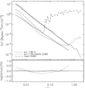
Figure 1. Q(r) andF(r) in 100 spherical radial bins about the most bound particle in haloG1from theL25 simulation atz=0. Top panel:Q(dot–
dashed curve); power-law fitQ∝r−1.84±0.012is given by upper thin solid
line.F(r) from EnBiD [withn= 10 smoothing kernel (dotted curve)]; power-law fit toF(r)∝r−1.59±0.054is given by lower thin solid line. Mean
value off(long-dashed curve) is noisier thanF(r) due to subhaloes. Resid-uals to the two power-law fits are shown in the bottom panel.
& Steinmetz (2006) showed that EnBiD with a kernel which in-cludes 10 nearest neighbours (n=10) about each point was able to recover analytic phase-space density profiles to nearly three to four decades higher values offthan FiEstAS.
For our haloes atz=0, the results we obtained with the different codes were completely consistent with those obtained by Sharma & Steinmetz (2006). The deviations between the estimates obtained with the different codes and various parameters were significantly higher at higher redshift – where comparisons with analytic esti-mates are not available. We refer the reader to the Appendix for a detailed comparison between estimated values off using the two codes at various redshifts. In the rest of this paper we present results obtained with EnBiD (n=10 kernel), the parameters preferred by Sharma & Steinmetz (2006).
Fig. 1 (top panel) shows the spherically averaged quantityQ= ρ/σ3 (dot–dashed curve), the mean off(x,v) in spherical bins (dashed curve) and the median DF in spherical bins (dotted curve). As we will show in Fig. 4, the large fluctuations in the mean value of
f(dashed curve) beyond 0.1rvirare due to the presence of substruc-ture, which can have extremely high central values off. The median value off(hereafter represented byF) is much smoother, being less sensitive to the large range (nearly eight orders of magnitude) infat each radius. In what follows, we will use the medianF, computed in concentric radial bins centred on the most bound particle in the main halo, since it is less sensitive to substructure.Q(r) is well fitted by a power law,Q∝r−1.84±0.012, over the radial range [0.004–0.6]r/r
vir (upper thin solid line). The power-law fitF(r)∝r−1.59±0.054over the same radial range is shown by the lower thin solid line. The bottom panel shows the residuals of the fitsF [log (F /Ffit)] and Q[log (Q/Qfit)]. This plot shows that whileQ(r) is an extremely
good power law, the medianF(r) is only approximately power law over the same radial range. Note thatQ(r) is numerically larger thanF(r) due to the fact that the former quantity does not properly account for the volume of the phase-space element. A similar result was obtained in a much higher resolution simulation by Stadel et al. (2008), a study which appeared as we were preparing this paper for publication.
3 E VO L U T I O N O F P H A S E - S PAC E D E N S I T Y W I T H R E D S H I F T
Hoffman et al. (2007) studied the phase-space density profiles of a DM halo by trackingQ(r) for material within the formal virial radius at each redshift. They found that the virialized material within this radius has an approximately power-law form with a constant power-law index of−1.9±0.05 at all redshifts fromz=5 to the present.
We follow a slightly different approach in this paper, since our objective is to understand the evolution of the true coarse-grained space density distribution. We track the evolution of phase-space density, by tracing backwards in time all the material that lies inside the virial radius atz=0. This will allow us to understand how the initially high phase-space density material that lies outside virialized systems at high redshift falls in and undergoes mixing and how the resultant mixing preserves the phase-space density profiles as a function of redshift.
We identified Milky Way sized DM haloes atz=0 in our cos-mological simulations and identify all the particles that lie inside twice the virial radius atz= 0. Our choice of halo outer radius (2rvir) is motivated by the recent work of Cuesta et al. (2008) who showed that the virial radius is arbitrary and does not correspond to a physically meaningful outer boundary for a DM halo. A better
outerradius is the so-called ‘static radius’, defined as the radius at which the mean radial velocity of particles is zero. This radius is typically about 2rvirfor a galaxy-sized DM halo. After identifying all particles within 2rviratz=0, we tracked them back toz=9. Our simulations do proceed back in time to even higher redshifts, however we do not analyse them here because the mass resolution at higher redshifts does not allow us to resolve the evolution of most of the objects beyond this epoch. There were 1.6×10⁶particles within 2 virial radii of theG1halo, which is the halo that is most isolated atz=0. Two other haloes (G2 andG3) from theL25 simulation are closer to each other atz=0 (1.5 virial radii apart). Therefore, we only tracked those particles which lay within one virial radius of the centres of these two haloes atz=0 back in time toz=9. The particles in the high-resolution simulationL20 were selected and tracked in the same way as for theG1halo, and atz=0 there were 3×10⁶particles inside twice the virial radius. The position and velocity data for all the particles identified as belonging to a given halo atz=0 were analysed.
At all redshifts we compute the phase-space densities of parti-cles inphysical coordinatesrather than in comoving coordinates. Distances are always in kpc and velocities are in km s−1, and these quantities are measured relative to the centre of the most massive progenitor. In many of the figures that follow, the physical distances at all redshifts other thanz=0 are scaled by the virial radius at
z=0, i.e. all distances are given in units ofr/rvir(z=0).
In this section, we will present the results obtained for the G1 halo in theL25 simulation. A comparison with results for the other three haloes is made in Section 4.
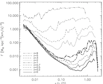
Figure 2.Fas a function of comoving radiusrfor all material that lies within 2rvirof the centre of theG1halo atz=0. Each curve corresponds to
a different redshift as indicated in the legends.
At the highest redshift plotted (z=9), the overall value ofFis higher at large radii than it is at the centre of the halo, and it only varies by a factor of a few over the entire range of radii [F∼10–30 Mkpc−3 (km s−1)−3]. This is because within the inner, virialized regions the coarse-grained phase-space density is lowered due to mixing, while it is still high in the outer regions where the large fraction of matter is not yet mixed or is located in small subhaloes that have not mixed to the same degree as the main host. As the evolution progresses, there is a decrease in the central value ofFtillz=3. The median
value ofFat the centre of the halo drops fromF≈10 Mkpc−3 (km s−1)−3atz=9 down toF≈2 M
kpc−3(km s−1)−3atz=0. The central value ofFremains constant beyondz=3, while there is a steady decrease inFat intermediate radii.
Although it is instructive to plot the mean and/or median values ofFat each radius, much more information is contained in the full coarse-grained phase-space densityf. The six-dimensional function
f(x,v) can be most easily visualized using the volume DFV(f), which also obeys a Mixing Theorem (Mathur 1988). Arad et al. (2004) showed that atz=0,V(f) for cosmological DM haloes follows a power-law profileV(f) ∝ f−α with power-law index α = 2.4 over four orders of magnitude in f. They argued that since DM haloes are almost spherical, if their phase-space DFs are approximately isotropic, their DFs could be written as functions of energy alone:f =f(E). In this case they showed that ifQ∝r−β, thenV(f) would also be described by a power law, and the indexα
was related to the indexβthrough a simple equation.
In Fig. 3, we plot the evolution ofV(f) with redshift for all the material that lies within twice the virial radius of haloG1atz=0. In the bottom-right panel, the solid line is a fit toV(f) for values of 10−4 < f <102.5. Over this range the best-fitting power-law profile is given byV(f)∝f−2.34±0.02which is not very different from the power-law profile fit obtained by Arad et al. (2004). At all redshifts,V(f) deviates from the power-law profile at both low and high end. It is likely that at the high-f end the distribution deviates from the power law due to the unresolved subhaloes below the mass resolution limit of the simulation.
TheMixing Theoremrequires that the coarse-grained volume DF
V(f) alwaysincreases(Mathur 1988). We see thatV(f) increases steadily fromz=9 onwards forf <1 Mkpc−3(km s−1)−3in such a way that as the system evolves, there is more volume associated with material with low f. At higher values of f, V(f) remains
Figure 4. Contours of constant particle number density in the plane [log (f), log (r)] for theG1halo, plotted at different redshifts. At each redshift the radial
distribution of particles is given relative to the most bound halo particle in units of the virial radius of the halo atz=0. The yellow and black contours correspond to the regions with the highest and lowest particle number densities, respectively. Contours are spaced at logarithmic intervals in particle number density relative to the maximum density contour.F, the median value offat each radius, is represented by the solid white line.
almost constant with decreasing redshift, probably owing to the fact that this material forms the cusps of DM haloes. While the Mixing Theorems have previously been demonstrated for isolated systems, this is to our knowledge the first demonstration of their validity in a cosmological context.
It is particularly illuminating to plot the full coarse-grained phase-space density of all particles as a function of radius from the centre of mass of the main halo at each redshift (Fig. 4). At any radius from the centre, there exist particles with phase-space densities spanning between four and eight decades inf. The coloured contours repre-sent a constant particle number per unit area on the plane [ log (f), log (r)]. The yellow/orange contours represent the parameter range with the largest number of particles, while the blue/black contours represent regions with the smallest number of particles. The solid white curves on each plot show the median value (F) off(x,v) in 100 logarithmically spaced bins inr. These curves are identical to the various curves in Fig. 2 and trace the regions with the largest particle number density at each radius. Numerous spikes inf are seen atr >0.1rvirand correspond to DM subhaloes.
As the evolution proceeds, there is an overall lowering of the me-dian phase-space densityF(white curves). There is also a continu-ous decrease of the low-end envelope offto lower values pointing to an increasingly large amount of matter with low phase-space den-sity. However, the upper envelope representing the highest phase-space density regions at the centres of the subhaloes remains rela-tively unchanged with redshift, indicating that primordial values of
fare largely preserved at the centres of DM subhaloes lying outside the centre of the main halo.
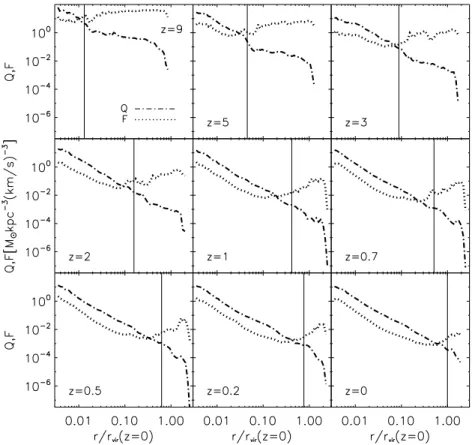
It is illustrative to compare the evolution ofF(r) andQ(r) with redshift. Fig. 5 shows the two curves plotted as a function of ra-dius (in comoving units) at each redshift for all the matter in halo
G1that lies within 2 virial radii atz= 0, as a function of phys-ical radius from the centre of the most massive progenitor of the final halo (in units of the virial radius atz=0). In each panel a thin vertical line is drawn atthe virial radius of the halo at that redshift.
We find the best-fitting power-lawQ∝r−1.84±0.012atz=0 to the profile within 0.6rvir. In agreement with Hoffman et al. (2007), we find that the same power law provides a reasonably good fit to the profiles at redshifts fromz∼5 to 0. WhileQalways decreases with radius since it is a spatial average over increasingly large volumes of configuration space, the median phase-space densityFdecreases monotonically with radius only within about 0.6rvirof the main pro-genitor at that redshift. Outside the virial radius at each redshift (i.e. to the right-hand side of the vertical dashed line),F(r) become sig-nificantly flatter, even increasing with increasing radius. At allz=
Figure 5. Q=ρ/σ3(dot–dashed line) and medianF(dotted line) as a function ofr/r
vir(z=0) for different redshifts for theG1halo. The dashed vertical
line is situated at the virial radius of the main halo at each redshift.
material in the subhalo centres, as well as in the relatively unmixed streams formed from disrupted subhaloes, prevents the median at large radii from decreasing rapidly, despite the large increase in low material with lowf-values within the virialized regions of the main halo.
To better understand the evolution offwith redshift we plot his-tograms of log (f) at each redshift in Fig. 6 (thick solid histograms). The thin red curves at each redshift represent the best-fitting Gaussians to the distribution of log (f) at that redshift. A Gaussian provides a good fit to the majority of the mass. [Since log (f) is close to Gaussian,fitself has a lognormal distribution.] By approximately
z=1, the skewness of the distribution is significant, and the skew-ness increases steadily untilz=0. To better understand the origin of the matter in the high-f tail atz=0, we plot the distribution of DM particles that have the values off≥1 Mkpc−3(km s−1)−3at
z=0. The ordinate values of this distribution (multiplied by a fac-tor of 10 to enhance visibility) are shown in the dashed histograms. The thin blue curves show that the high-ftail is also well fitted by a Gaussian (except atz=0). As we saw in Fig. 4, most of these high-f
tail particles are in subhaloes atz=0, while some are also in the highest phase-space density particles in the central cusp of the halo atz=0. This high-f subpopulation has a Gaussian distribution at
z=9 with a meanf=1.73±0.6 Mkpc−3(km s−1)−3compared with the meanf =1.57±0.54 Mkpc−3 (km s−1)−3for all the particles (in the solid curve) atz=9. A Student’st-test indicated with 99 per cent confidence that both distributions are drawn from the same population atz= 9. This implies that the material that lies in the centres of DM subhaloes atz=0 will have phase-space densities that are representative of the mean phase-space density of matter atz=9.
4 C O M PA R I S O N O F F O U R M I L K Y WAY S I Z E D H A L O E S
In this section we present results for the phase-space DFs for all four of the DM haloes described in Section 2. Although, we present results mainly atz=0, evolution with redshift for each of the haloes was similar to the evolution of haloG1presented earlier.
Fig. 7 compares the volume distribution of phase-space density
V(f) for the four different haloes atz=0. All three haloes from theL25 simulation (G1,G2,G3) show almost identical profiles in V(f) confirming the universality of the process that produced the phase-space DF. For haloL20,V(f) lies systematically above the other curves especially at higher values off, where it also extends to large values off. It was first shown by Sharma & Steinmetz (2006) that this is a numerical consequence of the increased mass resolu-tion of the simularesolu-tion. This indicates that the absolute value off
derived in the previous section is somewhat dependent on the mass resolution of the simulation and increases slightly with increasing mass resolution. In all four haloes,V(f) is well approximated by a power law over nearly six orders of magnitude inf. The first column of Table 1 gives details of the power law fits toV(f) (i.e. the power-law slopes and their errors over the range 10−4 < f < 102.5). The power-law slopes we obtained are similar to those ob-tained by previous authors (Arad et al. 2004).
In Fig. 8, we plotF(r) andQ(r) for the four different haloes atz=
0. The top set of four curves showQ(r) while the lower set of curves showF(r). In all four haloes,Q(r) is well fitted by a power law of slopeβ=1.8–1.9 (see Table 1).F(r) shows significant deviations from a simple power-law profile, with a systematic upturn beyond
Figure 6. Histograms of the phase-space densityf of all halo particles as a function of redshift (thick solid histograms). The dashed histograms follow those particles which have the highest phase-space densitiesf ≥1 atz=0, with ordinate values multiplied by 10 to enhance visibility. The thin red curves are the best-fitting Gaussians to all the particles in the thick solid histograms, while the thin blue curves are best-fitting Gaussians to dashed histograms.
Figure 7. V(f) for four haloes, atz=0. The triple-dot–dashed line is for G1, the dotted line forG2, the dashed line forG3and the solid line is for
higher mass resolution simulationL20.
have systematically higherFandQvalues than the haloes from the low-resolution simulation (again, a numerical consequence of the higher mass resolution; Sharma & Steinmetz 2006). Table 1 gives the values for the slopes and the error bars on the power law fits to
Q(r) andF(r) forr <0.6rviras well as the inner power-law slope ofF(r).
Table 1. Power-law indices for fits toV,QandFfor four haloes atz=0 forr <0.6rvir.
Halo V Q F
G1 −2.34±0.02 −1.84±0.01 −1.59±0.05
G2 −2.37±0.02 −1.82±0.01 −1.46±0.06
G3 −2.35±0.02 −1.75±0.01 −1.42±0.03
L20 −2.27±0.01 −1.87±0.01 −1.64±0.07
5 D I S C U S S I O N
Several previous studies have attempted to account for the origin of the power-lawQ(r) profiles of DM haloes. Notably, it has been ar-gued that power-law profiles result from virialization and not from the hierarchical sequence of mergers, since they are also produced in simple spherical gravitational collapse simulations (Taylor & Navarro 2001; Barnes et al. 2006, 2007). Our results presented in the previous section (Fig. 5) show that whileQ(r) andF(r) have approximately power-law form within 0.6rvir at a given redshift, F(r) flattens out and remains quite flat beyond this radius. Fur-thermore, as the hierarchical growth of the halo progresses these approximately power-law profiles extend to larger radii until they encompass all the mass within the virial radius atz=0.
Figure 8. Q(thin lines) andF(thick lines) for all the haloes studied, atz= 0. Triple-dot–dashed lines are forG1, dotted lines forG2, dashed lines for
G3and the solid lines forL20.
reasons for the preservation of the power-law profiles. First, the most tightly bound material – that forming a steep central cusp or shallow core—preserves its phase-space density in the final remnant. This is a consequence of the additivity of the excess mass function – a result of the fact that steeper cusps are less mixed than shallower cusps (Dehnen 2005). Over 60 per cent of the material in the central cusp (within one scale radius) of a progenitor NFW halo remains within the cusp of the merger remnant (Valluri et al. 2007). The second reason for preservation of power-law profiles at large radii is that material outside three scale radii of the progenitor haloes is redistributed to other radial bins almost uniformly from each radial interval. In addition, nearly 40 per cent of the material within the virial radius of the progenitor haloes is ejected to beyond the virial radius of the final remnant (Kazantzidis et al. 2006; Valluri et al. 2007). This material can be shown to have originated in roughly equal fractions from each radial interval beyond three scale radii and has higher phase-space density than expected from the simple power-law extrapolation of the inner power law. This self-similar redistribution of material contributes to the preservation of power-law profiles inQ(r) andF(r) in equal mass binary mergers. Thus, once a power-law phase-space DF has been established in a DM halo, major mergers will not destroy this profile. This has been con-firmed by our recent work on mergers of equal-mass haloes (Vass et al. 2009).
As discussed in the previous section (Fig. 6), the coarse-grained phase-space densityf in CDM haloes has a nearly lognormal distribution with the median of log (f) (the peak of the histogram
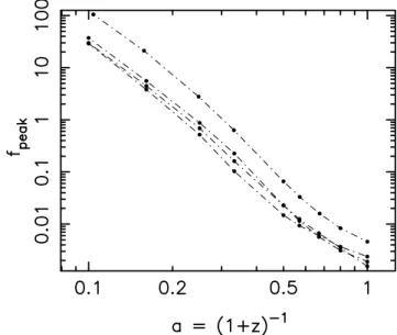
fpeak) evolving steadily towards lower values offas the halo grows. We now quantify the evolution offpeakwith redshift.
Fig. 9 shows the evolution of median phase-space densityfpeak derived from the histograms of log (f) in Fig. 6 for each of the four Milky Way sized cosmological haloes in this study. The solid dots represent the values of fpeak as a function a, while the dot–dashed curves are meant to guide the eye by con-necting points for each of the four individual haloes. Fora <
0.5 the decline infpeak is approximately power law, fpeak(a) ∝
a−4.5. This implies that the matter inside the haloes has un-dergone significant mixing due to virialization during the hi-erarchical formation process; the levelling off of the curve at
Figure 9. The median phase-space density (peak of histogramsfpeakin
Fig. 6) at each redshift as a function of the cosmic scalefactora=(1+ z)−1, plotted for four Milky Way sized haloes (points). The thin dot–dashed
curves connect points for the four individual haloes.
a∼ 0.5 indicates a decrease in mixing afterz =1, possibly re-sulting from a decrease in mass accreted in major mergers.
On average, as a halo grows via accretion its median density decreases as a power law with time, despite the fact that the most centrally concentrated material retains its original high phase-space density. This nearly power-law profile infpeakleads to some insights into the development of phase-space density profiles. We can break down the formation of haloes into two phases (Li et al. 2007): the fast accretion regime during which halo mass grows very rapidly and the slow accretion regime. In the fast accretion regime, the mixing processes are very efficient as the potential well is established and potential fluctuates rapidly and constantly. This results in a rapid decrease in the overall central phase-space density of the halo (as seen from the rapid drop in the central most regions of the profiles in Fig. 2). The inner profile of phase-space distribution should be largely set during this stage. As haloes grow subsequently, either by major mergers or by quiescent accretion of smaller haloes, the average phase-space density decreases, but the pre-existing high central phase-space density cusps are preserved.
At these later times the evolution of the true phase-space density is complex and occurs due to the accretion of high phase-space density material in subhaloes, as well as loosely bound material at the edges of the halo. The steady decrease in the amplitude and increase in the slope of the F(r) profiles in Fig. 2 with redshift show that the true phase-space density does not obey the power-law profiles seen inQ(r) at all redshifts. Variations in the individual power-law profiles of haloes both atz=0 (Fig. 8) and with redshift reflect the large variation in the cosmic accretion histories of individual haloes. Additional deviations from the power law arise due to the matter bound to subhaloes that survives with high phase-space density and leads to the variation of the coarse-grainedfof some six orders of magnitude in the outer regions of haloes.
the distribution of the coarse-grained phase-space density. TheQ
profile is a ratio of the density and velocity dispersion (which can be interpreted as a measure of temperature) and is therefore related to the entropy. For an ideal monatomic gas the entropy can be defined asKgas=T /ρ2/3, while for DM, by analogy, the entropy can be defined asKDM=σ2/ρ
2/3
DM(Faltenbacher et al. 2007). This, as noted by Hoffman et al. (2007), givesKDM∝Q−2/3orKDM∝
r1.2forQ∝r−1.8. This power-law form and slope of the entropy profile is very similar2 to the one found for the gas in the outer regions of clusters in cosmological simulations (e.g. Borgani et al. 2004; Voit, Kay & Bryan 2005). This power law is also predicted by the models of spherical accretion (Tozzi & Norman 2001) and reflects the increasing entropy to which the accreting material is heated as the halo grows its mass. Although the processes governing the virialization of gas and DM are different (the short-range local interactions for the former, and long-scale interactions for the latter), the fact that the resulting entropy profiles are quite similar indicates that they lead to the same distribution of entropy. TheQ(r) profile therefore may reflect the overall entropy profile of DM, not the coarse-grained local phase-space density, which exhibits a more complicated behaviour.
6 S U M M A R Y A N D C O N C L U S I O N S
We have investigated the evolution of the phase-space density of the DM in cosmological simulations of the formation of Milky Way sized DM haloes. The analysis was carried out using two different codes for estimating the phase-space density. Both codes give qualitatively similar results, but the estimated values of phase-space densityf are quite sensitive to the type of code and, for a given code, also depend quite sensitively on the choice of smoothing kernel used. Based on comparisons of the two codes (FiEstAS and EnBiD) and various smoothing parameters (see the Appendix), we select the EnBiD code withn=10 kernel smoothing and present results for the analysis with this set of parameters.
The simulations presented in this paper complement our analysis of the evolution of phase-space density in binary major mergers (Vass et al. 2009). We confirm that the profiles ofQ(r)=ρDM/σ3DM computed by previous authors can be described by a power law
Q(r)∝r−1.8±0.1over more than 2 orders of magnitude in radius in all haloes. The median of the phase-space density [F(r)] at given radius
r, however, exhibits a more complicated behaviour. AlthoughF(r) is approximately a power law forr <0.6rvir, the profiles generally flatten in the outer regions. Subhaloes contribute somewhat to this behaviour, although their effect is limited by the relatively small fraction of mass (<0.1) bound to them. However, in addition to subhaloes, a significant fraction of high phase-space density matter is in the relatively unmixed material (possibly in streams) arising from tidally disrupted subhaloes (e.g. Arad et al. 2004; Diemand et al. 2008). The rise inF(r) at large radii suggests that the fraction of mass in such streams can be substantial.
This behaviour holds at earlier epochs. Fromz=5 to 0, material within rvir(z) at each redshift follows a power law inQwith an approximate power-law slope of∼ −1.8 to−1.9. In contrast,F(r) can only be well described by a power law in the inner regions, and its slope changes continuously with redshift. Beyond the virial radius,Q(a quantity that is obtained by averaging over increasingly large volumes) decreases rapidly with radius, but the median value
2The slope is even more similar if one takes into account the random bulk
motions of the gas in estimatingKgas(Faltenbacher et al. 2007).
ofF flattens significantly. We argue thatF is a more physically meaningful quantity, especially for understanding the evolution of phase-space density in collisionless DM haloes, as it measures the median of the true coarse-grained phase-space density.
At all redshifts, the highest values of phase-space densityf are found at the centres of DM subhaloes. In the centre of the main halo, the median phase-space density (F) drops by about an or-der of magnitude from z = 9 to 0. In contrast, the centres of DM subhaloes maintain their high values off ∼103M
kpc−3 (km s−1)−3at all redshifts. The highest values off at the centre of the main halo are, therefore, lower and less representative of the pri-mordial phase-space density of DM particles than the central value offin the high phase-space density subhaloes. Atrvir, the decrease in median phase-space density is much more significant, withF≈
30 Mkpc−3 (km s−1)−3 at z = 9 decreasing to F ≈ 10−3M
kpc−3 (km s−1)−3 atz= 0, a decrease of over four or-ders of magnitude (Fig. 4).
The evolution ofF(r) andV(f) with redshift is consistent with expectations from the Mixing Theorems, which require that mixing reduces the overall phase-space density of matter in collisionless systems and that the volume of phase-space associated with any value offincreases due to mixing and relaxation.
The distribution of f is approximately lognormal untilz ∼3. As time progresses, the mean and median of log (f) shift to pro-gressively lower values as a larger and larger fraction of matter undergoes mixing and moves to lower values off. Some fraction of high phase-space density material does survive in the centres of subhaloes and in the relatively unmixed streams leftover after subhalo disruptions, which skews the distribution. Remarkably, the highest phase-space density particles atz=0 have retained their phase-space density sincez≈9, the earliest epoch we analysed. The phase-space density in the centres of DM subhaloes is therefore representative of the mean phase-space density of DM at the high-est redshifts. This can potentially allow for stronger constraints to be placed on the nature of DM particles from the Tremaine–Gunn bound (Tremaine & Gunn 1979; Hogan & Dalcanton 2000).
The median value of phase-space density decreases with de-creasing redshift approximately as a power law described by
fpeaka−4.5. This majority of the decrease infpeakis the result of mixing within virialized haloes which reduces the coarse-grained phase-space density of matter that has turned around from the Hub-ble flow; much of this mixing occurs prior toz∼1, after which the rate of mixing in galactic-sized haloes slows down.
AC K N OW L E D G M E N T S
Institute for Theoretical Physics, supported in part by the NSF un-der grant PHY05-51164, for hospitality during the final editing of the paper and participants of the workshop ‘Back to the Galaxy’ for useful discussions and feedback on the results of this paper. SK is supported by the Center for Cosmology and Astro-Particle Physics (CCAPP) at The Ohio State University.
R E F E R E N C E S
Arad I., Dekel A., Klypin A., 2004, MNRAS, 353, 15 Ascasibar Y., Binney J., 2005, MNRAS, 356, 872
Ascasibar Y., Yepes G., Gottl¨ober S., M¨uller V., 2004, MNRAS, 352, 1109 Austin C. G., Williams L. L. R., Barnes E. I., Babul A., Dalcanton J. J.,
2005, ApJ, 634, 756
Barnes E. I., Williams L. L. R., Babul A., Dalcanton J. J., 2006, ApJ, 643, 797
Barnes E. I., Williams L. L. R., Babul A., Dalcanton J. J., 2007, ApJ, 654, 814
Bertschinger E., 1985, ApJS, 58, 39
Binney J., Tremaine S., 1987, Galactic Dynamics. Princeton Univ. Press, Princeton, NJ, p. 747
Borgani S. et al., 2004, MNRAS, 348, 1078
Cuesta A. J., Prada F., Klypin A., Moles M., 2008, MNRAS, 389, 385 Dehnen W., 2005, MNRAS, 360, 892
Dehnen W., McLaughlin D. E., 2005, MNRAS, 363, 1057
Diemand J., Kuhlen M., Madau P., Zemp M., Moore B., Potter D., Stadel J., 2008, Nat, 454, 735
Faltenbacher A., Hoffman Y., Gottl¨ober S., Yepes G., 2007, MNRAS, 376, 1327
Gnedin N. Y., Kravtsov A. V., 2006, ApJ, 645, 1054
Hoffman Y., Romano-D´ıaz E., Shlosman I., Heller C., 2007, ApJ, 671, 1108
Hogan C. J., Dalcanton J. J., 2000, Phys. Rev. D, 62, 063511 Kazantzidis S., Zentner A. R., Kravtsov A. V., 2006, ApJ, 641, 647 Klypin A., Zhao H., Somerville R. S., 2002, ApJ, 573, 597 Knollmann S. R., Knebe A., Hoffman Y., 2008, MNRAS, 391, 559 Kravtsov A. V., Klypin A. A., Khokhlov A. M., 1997, ApJS, 111, 73 Kravtsov A. V., Gnedin O. Y., Klypin A. A., 2004, ApJ, 609, 482 Li Y., Mo H. J., van den Bosch F. C., Lin W. P., 2007, MNRAS, 379,
689
Maciejewski M., Colombi S., Alard C., Bouchet F., Pichon C., 2009, MNRAS, 393, 703
Mathur S. D., 1988, MNRAS, 231, 367
Merritt D., Graham A., Moore B., Diemand J., Terzi´c B., 2006, AJ, 132, 2685
Navarro J. F., Frenk C. S., White S. D. M., 1996, ApJ, 462, 563
Rasia E., Tormen G., Moscardini L., 2004, MNRAS, 351, 237 Sharma S., Steinmetz M., 2006, MNRAS, 373, 1293
Stadel J., Potter D., Moore B., Diemand J., Madau P., Zemp M., Kuhlen M., Quilis V., 2008, MNRAS, submitted (arXiv:0808.2981)
Taylor J. E., Navarro J. F., 2001, ApJ, 563, 483 Tozzi P., Norman C., 2001, ApJ, 546, 63
Tremaine S., Gunn J. E., 1979, Phys. Rev. Lett., 42, 407
Tremaine S., Henon M., Lynden-Bell D., 1986, MNRAS, 219, 285 Valluri M., Vass I. M., Kazantzidis S., Kravtsov A. V., Bohn C. L., 2007,
ApJ, 658, 731
Vass I. M., Kazantzidis S., Valluri M., Kravtsov A. V., 2009, ApJ, in press (arXiv:0812.3659)
Vogelsberger M., White S. D. M., Helmi A., Springel V., 2008, MNRAS, 385, 236
Voit G. M., Kay S. T., Bryan G. L., 2005, MNRAS, 364, 909 Wang J., White S. D. M., 2008, MNRAS, submitted (arXiv:0809.1322) Wojtak R., Łokas E. L., Mamon G. A., Gottl¨ober S., Klypin A., Hoffman
Y., 2008, MNRAS, 388, 815
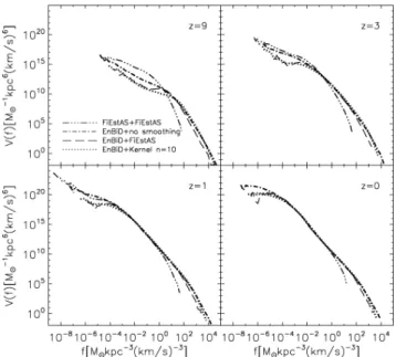
Figure A1. The volume DFV(f) at different redshifts during the evolution of theG1halo in theL25 simulation. Plots compare results obtained with
the FiEstAS code and EnBiD code (using three different parameters) as indicated in the line legends.
A P P E N D I X A : C O M PA R I S O N O F ‘ F I E S T A S ’ A N D ‘ E N B I D ’ A N A LY S I S O F H A L O G1
The numerical estimation of coarse-grained phase-space densities during the evolution of the fourN-body haloes presented in this paper was carried out using two publicly available codes ‘FiEstAS’ (Ascasibar & Binney 2005) and ‘EnBiD’ (Sharma & Steinmetz 2006). A comparison of these two codes has previously been pre-sented by Sharma & Steinmetz (2006), who showed for an analytic DF (for the spherical Hernquist potential), that ‘EnBiD withn=10 kernel smoothing’ gave the highest fidelity to the analytical DF. In a related work, Vass et al. (2009) confirmed the findings of Sharma & Steinmetz (2006) for a spherical isotropic NFW halo. This latter study is the main basis for our choice of EnBiD withn=10 kernel smoothing. After this paper was submitted to the Journal we be-came aware of the work of Maciejewski et al. (2008). These authors carried out a similar, and somewhat more detailed, comparison of coarse-grained phase-space density estimators forN-body simula-tions on cosmological haloes atz=0. Our results are in agreement with theirs.
However, it is unclear whether the comparisons with analytic profiles of isolated haloes atz=0 are valid for matter distributions arising from cosmologicalN-body distributions, at high redshifts, where the majority of the particles actually lie outside virialized haloes. Our purpose in this Appendix is to present a comparison of results obtained with the different codes at a range of redshifts to allow readers to appreciate how sensitive some of the results presented in this paper are to the choice of code and smoothing parameters used in density estimation. Since the coarse-grained DF
Table A1. Power-law indicesV(f)∝f−αandF(r)∝r−β atz=0 from different codes.
Code α β
FiEstAS 2.62±0.06 1.43±0.02
EnBiD (no smoothing) 2.35±0.02 1.65±0.02 EnBiD (FiEstAS smoothing) 2.46±0.03 1.69±0.07 EnBiD (kerneln=10) 2.34±0.02 1.59±0.05
(long-dashed curves) and EnBiD with an n =10 kernel (dotted curves). In each case we see thatV(f) has a nearly power-law dis-tribution over more than six orders of magnitude infatz=0 [from ∼10−4to 103M
kpc−3 (km s−1)−3]. Table A1 gives the slopes of power-law fits for the four different estimates ofV(f) over the range 10−4 < f <103 atz=0. The FiEstAS estimate ofV(f) is systematically lower than all EnBiD estimates at high values of
f (at all redshifts). In addition, all EnBiD curves extend to much higher values off than the FiEstAS estimate (this is particularly true atz=9 where the FiEstAS estimate differs from the other es-timates both quantitatively and qualitatively). The results from the various EnBiD estimates differ very little at intermediate values of
f (10−4–103), and consequently we are confident that conclusions drawn from the medianfare quite insensitive to the details of the EnBiD parameters used to obtainf.
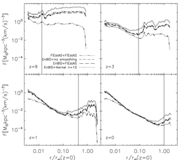
The differences between the various estimates ofFat large radii become significantly larger at higher redshift. In Fig. A2, we plot the four different estimates ofF(r) at four different redshifts in the evolution. The vertical dashed line in each panel represents the virial radius of the main halo at that redshift. We see thatFfrom any of the codes is quite flat beyond the virial radius in all cases, but the absolute values of the curves differ significantly. Note that atz=9, the different estimates can differ by as much as two orders of magnitude.
Figure A2. Ffor theG1halo in theL25 simulation at different redshifts
obtained using FiEstAS and EnBiD as indicated by line-legends. The dashed vertical line is situated at the virial radius of the main halo at each redshift.
In this paper, we choose to present results from EnBiD withn=
10 kernel smoothing over the other estimates largely because it does the best job of reproducing analytic DFs (Sharma & Steinmetz 2006) and because it appears to provide a good upper limit to the phase-space density both at high and at low values off. In the absence of an analytic comparison of the estimates at high redshift, we caution the reader to refrain from drawing very strong conclusions regarding absolute values offorFfrom the results presented here.
![Figure 4. Contours of constant particle number density in the plane [log (f ), log (r)] for the G 1 halo, plotted at different redshifts](https://thumb-us.123doks.com/thumbv2/123dok_us/102512.1015409/6.892.207.680.79.525/figure-contours-constant-particle-density-plotted-different-redshifts.webp)