R E S E A R C H
Open Access
New results on reachable set bounding for
linear time delay systems with polytopic
uncertainties via novel inequalities
Hao Chen
1,2*and Shouming Zhong
2*Correspondence: [email protected]
1School of Mathematical Sciences, Huaibei Normal University, Huaibei, 235000, China
2School of Mathematical Sciences, University of Electronic Science and Technology of China, Chengdu, 611731, China
Abstract
This work is further focused on analyzing a bound for a reachable set of linear uncertain systems with polytopic parameters. By means of L-K functional theory and novel inequalities, some new conditions which are expressed in the form of LMIs are derived. It should be noted that novel inequalities can improve upper bounds of Jensen inequalities, which yields less conservatism of systems. Consequently, some numerical examples demonstrate that the authors’ results are somewhat more effective and advantageous compared with the previous results.
Keywords: reachable set; polytopic uncertainties; Lyapunov-Krasovskii (L-K) functional; linear matrix inequality (LMI)
1 Introduction
It is well known that reachable set estimation was first researched in the late s for state estimations. The reachable set is a hot issue since the time due to its important and wide application in the design of controller and aircraft collision avoidance and peak-to-peak gain minimization problems. The reachable set of dynamic differential systems with delay and disturbance is a set that contains all the reachable trajectories from origin by outside peak input values [–]. In the real world, as for dynamic systems, there are two phenomena that cannot be avoided: time delays and uncertainties [–]. In fact, delays and the coefficients of differential equations in modeling progresses are obtained only ap-proximately [–]. There are already some relevant outstanding results about reachable set estimation of dynamic systems. However, we think it is necessary to obtain a more tighter bound for a reachable set.
As pointed out in [–], an equation of one class can be transformed to an equation belonging to the external form of the other class. Thus, it is natural to classify the equa-tions according to the properties of operators generated by the equaequa-tions. In this paper, uncertain polytopic delayed linear systems with disturbances will be studied.
All the results about reachable set bounding are in the term of linear matrix inequali-ties (LMIs). The authors give an ellipsoid condition of the reachable set for linear systems without any delay []. The authors Fridman and Shaked improved the model []. They studied the linear systems with varying delays with peak inputs and got LMIs conditions of an ellipsoid by using the Razumikhin theory. After that, Kim got a more exact condition
by constructing the modified Lyapunov-Razumikhin functionals []. Combining the de-composition technique, Nam derived a modified reachable set bound []. Actually, the reachable set is not an ellipsoid and it is only a closed set. Zuo et al. gave a non-ellipsoidal bound of a reachable set for linear time-delayed systems by the means of the maximal Lyapunov functionals and the Razumikhin method [].
It should be noted that discrete delay is varying ≤τ(t)≤τin most previous literature. That is, the lower bound of discrete delay is . In fact,τ(t) varyingτm≤τ(t)≤τM may
describe the delay more exactly. In order to control the behavior of the system better, we hope to propose tighter reachable set estimation. Park, Lee and Lee proposed some novel inequalities which can be used to estimate integrations []. Therefore, those inequalities can be employed to estimate some integration terms of Lyapunov functionals for dynamic systems. Motivated by the above mentioned discussions, we consider the linear time-varying delay systems with polytopic uncertainties. Using novel inequalities, we derive a modified reachable set bound for the linear system with discrete delayτm≤τ(t)≤τM.
Moreover, four examples are given to demonstrate the effectiveness and advantage of our results.
In this paper, the used notations are listed as follows. Real matrixP> (≥) denotes thatPis a symmetric positive definite matrix (positive semi-definite). Superscript ‘T’ is transposition of a vector and a matrix;∗means the elements below the main diagonal in a symmetric block matrix;Iis an identity matrix; ‘–’ in tables means that there is no feasible solution for linear matrix inequalities.
2 Preliminaries
Consider uncertain polytopic delayed linear systems with disturbances in the form
˙
z(t) = (A+A)z(t) + (D+D)zt–τ(t)+ (B+B)w(t),
z(t) = , t∈[–τM, ],
()
wherez(t)∈Rnis a state vector;w(t)∈Rmis outside disturbance.A,A∈Rn×n,D,D∈ Rn×n,B,B∈Rn×m.A,D,Bare known matrices.A,D,Bare uncertain matrices.τ(t)
is time delay.
Discrete delayτ(t) and disturbancew(t) are assumed to be as follows:
τm≤τ(t)≤τM, ≤ ˙τ(t)≤μ< ,
wT(t)w(t)≤wm, whereμ,wmare constant.
The uncertainty parameter matrices are expressed by a linear convex-hull of matrices Ai,BiandDi
A=
N
i=
θi(t)Ai, B= N
i=
θi(t)Bi, D= N
i=
θi(t)Di
withθi(t)∈[, ] and
N
i=θi(t) = ,∀t> .Ai,BiandDiare known matrices.
Lemma ([]) As for the well-defined integralab((tt))f(t,s)ds,the following relation known as the Leibniz rule holds:
d dt
b(t)
a(t)
f(t,s)ds=b(t)f˙ t,b(t) –a(t)f˙ t,a(t) +
b(t)
a(t)
∂
∂tf(t,s)ds.
Lemma ([]) For a positive definite matrix R> and a differentiable function{z(u)|u∈ [a,b]},the following inequalities hold:
(b–a)
b
a
zT(s)Rz(s)ds≥ξT
R –R
∗ R
ξ,
(b–a)
b
a
˙
zT(s)Rz(s)˙ ds dθ≥ξT ⎡ ⎢ ⎢ ⎢ ⎣
R –R R –R
∗ R –R R
∗ ∗ R –R
∗ ∗ ∗ R
⎤ ⎥ ⎥ ⎥ ⎦ξ,
b
a
b
θ
˙
zT(s)Rz(s)˙ ds dθ≥ξT ⎡ ⎢ ⎣
R R –R
∗ R –R
∗ ∗ R
⎤ ⎥ ⎦ξ,
where
ξT=
b–a
b
a
zT(s)ds, (b–a)
b
a
b
θ
zT(s)ds dθ
,
ξT=
zT(b),zT(a), b–a
b
a
zT(s)ds, (b–a)
b
a
b
θ
zT(s)ds dθ
,
ξT=
zT(b), b–a
b
a
zT(s)ds, (b–a)
b
a
b
θ
zT(s)ds dθ
.
Lemma ([]) Let V be a Lyapunov function for system()with wT(t)w(t)≤w
m.If
˙
V+αV– α w
m
wT(t)w(t)≤,
then V≤.
3 Main results
In this section, we will firstly consider a reachable set for uncertain parameter matrices
A= ,D= ,B= in system (), namely,
˙
z(t) =Az(t) +Dzt–τ(t)+Bw(t), z(t) = , t∈[–h, ]. ()
After that, we will consider a reachable set for uncertain system ().
Ifτm≤τ(t)≤τM,τ˙(t)≤μ< , we get the reachable set bounding for dynamic system
() in Theorem .
α> such that the following inequality holds:
= ⎡ ⎢ ⎢ ⎢ ⎢ ⎢ ⎢ ⎢ ⎢ ⎢ ⎢ ⎢ ⎢ ⎢ ⎢ ⎢ ⎢ ⎢ ⎢ ⎣
∗ ∗ ∗ , ∗ ∗ ∗ ,
∗ ∗ ∗ ∗
∗ ∗ ∗ ∗ ∗
∗ ∗ ∗ ∗ ∗ ∗ ,
∗ ∗ ∗ ∗ ∗ ∗ ∗
∗ ∗ ∗ ∗ ∗ ∗ ∗ ∗
∗ ∗ ∗ ∗ ∗ ∗ ∗ ∗ ∗
∗ ∗ ∗ ∗ ∗ ∗ ∗ ∗ ∗ ∗
∗ ∗ ∗ ∗ ∗ ∗ ∗ ∗ ∗ ∗ ∗
⎤ ⎥ ⎥ ⎥ ⎥ ⎥ ⎥ ⎥ ⎥ ⎥ ⎥ ⎥ ⎥ ⎥ ⎥ ⎥ ⎥ ⎥ ⎥ ⎦
≤, ()
where
=αP+PA+ATP+R+M– e–ατmQ– e–ατmM – e–ατMM
+NA+ATNT+ATNA+ATNTA,
=PD+ND+ATND+ATNTD, = e–ατmQ,
= –e–ατmQ– e–ατmM, = –e–ατMM,
= e–ατmQ+ e–ατmM,
= e–ατMM, = –N–ATNT–ATN,
=PB+NB+ATNB+ATNTB,
= –( –μ)e–ατMM+DTND+DTNTD,
= –DTNT–DTN, =DTNB+DTNTB,
=e–ατmR–e–ατmR– e–ατmQ– e–ατMQ,
= e–ατMQ, = e–ατmQ, = –e–ατMQ,
= –e–ατmQ, = e–ατMQ,
= –e–ατMR– e–ατMQ, = e–ατMQ, = –e–ατMQ,
= –e–ατmQ– e–ατmM, = e–ατmQ+ e–ατmM,
= –e–ατMM, = e–ατMM,
= –e–ατMQ, = e–ατMQ,
= –e–ατmQ– e–ατmM,
= –e–ατMM, = –e–ατMQ,
= (τm)Q+ (τM–τm)Q+N+NT, = –NB–NTB,
= –
α
w
m
Then the reachable sets of system()are bounded in a ball B(,r) ={z∈Rn|z ≤r}with
r=√
λmin(P)
. ()
Proof Construct the Lyapunov-Krasovskii functional
V(zt) =
i= Vi(zt),
where
V(zt) =zT(t)Pz(t),
V(zt) =
t
t–τm
eα(s–t)zT(s)Rz(s)ds+
t–τm
t–τM
eα(s–t)zT(s)Rz(s)ds,
V(zt) =
t
t–τ(t)
eα(s–t)zT(s)Mz(s)ds,
V(zt) =τm
–τm
t
t+θ
eα(s–t)z˙T(s)Q˙z(s)ds,
V(zt) = (τM–τm)
–τm
–τM
t
t+θ
eα(s–t)z˙T(s)Q˙z(s)ds,
V(zt) =
t
t–τm
t
θ
t
λ
eα(s–t)˙zT(s)M
z(s)˙ ds dθdλ
+
t
t–τM
t
θ
t
λ
eα(s–t)z˙T(s)M
z(s)˙ ds dθdλ.
Computing the derivative ofV(zt) of model (), we have
˙
V(zt) = zT(t)Pz(t) = –˙ αV(zt) + zT(t)P˙z(t) +αzT(t)Pz(t)
= –αV(zt) +αzT(t)Pz(t) + zT(t)P
Az(t) +Dzt–τ(t)+Bw(t), ()
˙
V(zt) = –αV(zt) +zT(t)Rz(t) +e–ατmzT(t–τm)Rz(t–τm)
–e–ατmzT(t–τ
m)Rz(t–τm) –e–ατMzT(t–τM)Rz(t–τM), ()
˙
V(zt) = –αV(zt) +zT(t)Mz(t) –
–τ˙(t)e–ατ(t)zTt–τ(t)Mz
t–τ(t)
≤–αV(zt) +zT(t)Mz(t) – ( –μ)e–ατMzT
t–τ(t)Mz
t–τ(t), ()
˙
V(zt) = –αV(zt) +τm˙zT(t)Qz(t) –˙ τm
t
t–τm
eα(s–t)˙zT(s)Qz(s)˙ ds
≤–αV(zt) +τmz˙T(t)Qz(t) –˙ e–ατmτm
t
t–τm
By using Lemma ,
˙
V(zt)≤–αV(zt) +τmz˙T(t)Qz(t)˙
–e–ατmζT ⎡ ⎢ ⎢ ⎢ ⎣
Q –Q Q –Q
∗ Q –Q Q
∗ ∗ Q –Q
∗ ∗ ∗ Q
⎤ ⎥ ⎥ ⎥
⎦ζ, ()
whereζT= (zT(t),zT(t–τ m),τm
t t–τmz
T(s)ds, τm
t t–τm
t
θzT(s)ds dθ),
˙
V(zt)
= –αV(zt) + (τM–τm)z˙T(t)Qz(t) – (˙ τM–τm)
t–τm
t–τM
eα(s–t)˙zT(s)Qz(s)˙ ds ≤–αV(zt)
+ (τM–τm)z˙T(t)Q˙z(t) –e–ατM(τM–τm)
t–τm
t–τM
eα(s–t)˙zT(s)Qz(s)˙ ds. ()
By using Lemma ,
˙
V(zt)≤–αV(zt) + (τM–τm)z˙T(t)Qz(t)˙
–e–ατMζT ⎡ ⎢ ⎢ ⎢ ⎣
Q –Q Q –Q
∗ Q –Q Q
∗ ∗ Q –Q
∗ ∗ ∗ Q
⎤ ⎥ ⎥ ⎥
⎦ζ, ()
where
ζT=
zT(t–τm),zT(t–τM),
τM–τm
t–τm
t–τM
zT(s)ds, (τM–τm)
t–τm
t–τM
t–τm
θ
zT(s)ds dθ
,
˙
V(zt) = –αV(zt) +
τ
m˙z(t)Mz(t) +˙ τ
Mz(t)M˙ ˙z(t) –
t
t–τm
t
θ
eα(s–t)z˙T(s)M
z(s)˙ ds dθ–
t
t–τM
t
θ
eα(s–t)˙zT(s)M
˙z(s)ds dθ
≤–αV(zt) +
τ
mz(t)M˙ z(t) +˙ τ
Mz(t)M˙ z(t)˙ – e–ατm
t
t–τm
t
θ
˙
zT(s)Mz(s)˙ ds dθ
– e–ατM
t
t–τM
t
θ
˙
In the light of Lemma ,
˙
V(zt)≤–αV(zt) +
τ
mz(t)M˙ z(t) +˙ τ
Mz(t)M˙ z(t)˙
– e–ατmζT
⎡ ⎢ ⎣
M M –M
∗ M –M
∗ ∗ M
⎤ ⎥ ⎦ζ
– e–ατMζT
⎡ ⎢ ⎣
M M –M
∗ M –M
∗ ∗ M
⎤ ⎥
⎦ζ, ()
where
ξT=
zT(t),
τm
t
t–τm
zT(s)ds,
τ
m
t
t–τm
t
θ
zT(s)ds dθ
,
ξT=
zT(t),
τM
t
t–τM
zT(s)ds,
τM
t
t–τM
t
θ
zT(s)ds dθ
.
Certainly, the following equations hold:
–˙z(t) +Az(t)
+Dzt–τ(t)+Bw(t)TN
–˙z(t) +Az(t) +Dzt–τ(t)+Bw(t)= ,
zT(t)N
–˙z(t) +Az(t) +Dzt–τ(t)+Bw(t)= ,
()
whereN,Nare matrices with appropriate dimensions. Through ()-() and ()()()(), one gets
˙
V(zt) +V˙(zt) +V˙(zt) +V˙(zt) +V˙(zt) +V˙(zt) –
α
w
m
wT(t)w(t)
≤–αV(zt) –αV(zt) –αV(zt) –αV(zt) –αV(zt) –αV(zt) +ζT(t)ζ(t).
That is,
˙
V(zt) –
α
w
m
wT(t)w(t)≤–αV(zt) +ζT(t)ζ(t).
Then one has
˙
V(zt) +αV(zt) –
α
w
m
wT(t)w(t)≤ζT(t)ζ(t), ()
where
ζT(t) =
zT(t),zTt–τ(t),zT(t–τm),zT(t–τM),
τm
t
t–τm
zT(s)ds,
τM
t
t–τM
zT(s)ds,
τM–τm
t–τm
t–τM
zT(s)ds,
τ
m
t
t–τm
t
θ
zT(s)ds dθ,
τM
t
t–τM
t
θ
zT(s)ds dθ, (τM–τm)
t–τm
t–τM
t–τm
θ
zT(s)ds dθ,z˙T(t),wT(t)
.
For () holding, we getV˙ +αV– α
wmw
Thus, according to Lemma , one hasV(zt)≤.
It is easy to see
zT(t)Pz(t) =V(zt)≤V(zt) +V(zt) +V(zt) +V(zt) +V(zt) +V(zt) =V(zt).
Furthermore, by using the spectral property for symmetric positive definite matrixP, we get
λmin(P)z(t)≤V(zt). ()
Therefore,z(t) ≤r=√ λmin(P)
due to ().
Next, let us consider the polytopic uncertain linear system (). Reachable set bounding of system () is got and stated in Theorem .
Theorem If there exist appropriate dimension matrices P> ,R> ,R> ,Q> , Q> ,M > ,M> ,M> ,appropriate dimensions matrices N,N,and a scalar
α> ,such that the following inequalities hold(i= , , . . . ,N):
i=
⎡ ⎢ ⎢ ⎢ ⎢ ⎢ ⎢ ⎢ ⎢ ⎢ ⎢ ⎢ ⎢ ⎢ ⎢ ⎢ ⎢ ⎢ ⎢ ⎣
i i i i i i i i i
∗ i i i
∗ ∗ i i i i i ,i
∗ ∗ ∗ i i ,i
∗ ∗ ∗ ∗ i i
∗ ∗ ∗ ∗ ∗ i i
∗ ∗ ∗ ∗ ∗ ∗ i ,i
∗ ∗ ∗ ∗ ∗ ∗ ∗ i
∗ ∗ ∗ ∗ ∗ ∗ ∗ ∗ i
∗ ∗ ∗ ∗ ∗ ∗ ∗ ∗ ∗ i
∗ ∗ ∗ ∗ ∗ ∗ ∗ ∗ ∗ ∗ i i
∗ ∗ ∗ ∗ ∗ ∗ ∗ ∗ ∗ ∗ ∗ i
⎤ ⎥ ⎥ ⎥ ⎥ ⎥ ⎥ ⎥ ⎥ ⎥ ⎥ ⎥ ⎥ ⎥ ⎥ ⎥ ⎥ ⎥ ⎥ ⎦
≤, ()
where
i=αPi+Pi(A+Ai) + (A+Ai)TPi+R+M– e–ατmQ– e–ατmM– e–ατMM +N(A+Ai) + (A+Ai)TNT+ (A+Ai)TN(A+Ai) + (A+Ai)TNT(A+Ai),
i=Pi(D+Di) +N(D+Di) + (A+Ai)TN(D+Di) + (A+Ai)TNT(D+Di),
i= e–ατmQ, i= –e–ατmQ– e–ατmM,
i= –e–ατMM, i= e–ατmQ+ e–ατmM,
i= e–ατMM, i= –N– (A+Ai)TNT– (A+Ai)TN,
i=Pi(B+Bi) +N(B+Bi) + (A+Ai)TNB+ (A+Ai)TNT(B+Bi),
i= –( –μ)e–ατMM+ (D+Di)TN(D+Di) + (D+Di)TNT(D+Di),
i= –(D+Di)TNT– (D+Di)TN, i= (D+Di)TNB+ (D+Di)TNTB
i= e–ατMQ, i= e–ατmQ, i= –e–ατMQ,
i= –e–ατmQ, i= e–ατMQ,
i= –e–ατMR– e–ατMQ, i= e–ατMQ, i= –e–ατMQ,
i= –e–ατmQ– e–ατmM, i= e–ατmQ+ e–ατmM,
i= –e–ατMM, i= e–ατMM,
i= –e–ατMQ, i= e–ατMQ,
= –e–ατmQ– e–ατmM,
= –e–ατMM, i= –e–ατMQ,
i= (τm)Q+ (τM–τm)Q+N+NT, i= –N(B+Bi) –NT(B+Bi),
i= –
α
w
m
+ (B+Bi)TN(B+Bi) + (B+Bi)TNT(B+Bi).
Then the reachable sets of system()are bounded in a ball B(,r) ={z∈Rn|z ≤r}with
r=√
λmin(Pi)
, i= , , . . . ,n. ()
Proof In progress in Theorem , replacing matrixAby Ni=θi(t)(A+Ai), matrixBby
N
i=θi(t)(B+Bi), matrixDby
N
i=θi(t)(D+Di), one can easily get the conclusion.
Remark In this paper, the discrete delayτm≤τ(t)≤τMis of a more general scope than
≤τ(t)≤τconsidered in [, , ].
Remark The novel inequalities in Lemma lead to tighter bounds than the Jensen in-equality. By means of novel inequalities in Lemma , to estimate integral terms in Lya-punov functionals, better bounds for a reachable set are proposed in this paper.
Remark To compute the smallest bound of a reachable set for linear dynamic systems (), we solve the optimization problem for a positive scalarδ> :
min δ¯
¯
δ=
δ
s.t.
⎧ ⎨ ⎩
(a) P≥δI,
(b) inequality ()/() in Theorem /.
()
Remark The novel inequalities in Lemma may be used to study the reachable set
problem for a linear neutral system, even for a non-linear neutral system.
Remark In references [, , ], they used conventional Jensen inequalities –(h– h)
t–h
t–h z
T(s)Pz(s)ds≤–(t–h
t–h z(s)ds)
TP(t–h
t–h z(s)ds) and –
(h–h)
–h
–h
t–h
t+θ zT(s)× Rz(s)ds dθ ≤ –(–h
–h
t–h
t+θ zT(s)ds dθ)R(
–h
–h
t–h
bound in this study is more accurate than those in references. Therefore, the conservatism in our work is less than the existing ones.
Remark It should be noted that if there are more accurate inequalities to estimate the
bound ofabzT(s)Rz(s)ds,b
a z˙T(s)R˙z(s)ds dθ,
b a
b
θ ˙zT(s)Rz(s)˙ ds dθ, there is still room for further improvement of the proposed results to reduce the conservatism of systems.
Remark Some literature works researched the stability of second order delay
differen-tial equations; see, for example, references [–]. In the future, reachable set bounding for second order delay differential equations may be a hot issue, and methods similar to those in this paper may be used to estimate reachable set bounding for second order delay differential equations.
4 Examples
In order to compare the obtained results with those in the literature, we provide several numerical examples in the following.
Example Consider the uncertain time-varying delayed system in [, ]:
A+A=
– –.
, A+A=
– –.
, D+D=
– – –.
,
D+D=
– – –.
, B+B=
–.
=B+B, wT(t)w(t)≤.
()
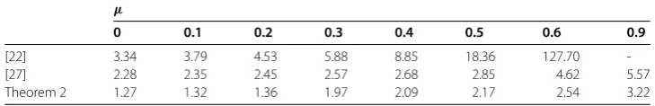
[image:10.595.133.481.365.439.2]We consider two cases for discrete delayτ(t): ≤τ(t)≤.,τ˙(t)≤μ< and ≤τ(t)≤ .,τ˙(t)≤μ< . Letμbe different values, we computeδ¯’s by using optimization problem (). The computedδ¯’s are listed in Table for the forward case and in Table for the backward case. From Tables and , we know that the proposed result in Theorem is tighter than the ones in references [, ].
Table 1 δ¯’s in Example 1 for 0≤τ(t)≤0.7,τ˙(t)≤μ
μ
0 0.1 0.2 0.3 0.4 0.5 0.6 0.9
[22] 2.97 3.30 3.85 4.85 6.93 12.84 53.86
-[27] 1.89 1.94 2.00 2.08 2.19 2.35 2.60 3.51
[image:10.595.115.480.673.732.2]Theorem 2 1.38 1.51 1.59 1.63 1.70 1.81 1.94 2.05
Table 2 δ¯’s in Example 1 for 0≤τ(t)≤0.75,τ˙(t)≤μ
μ
0 0.1 0.2 0.3 0.4 0.5 0.6 0.9
[22] 3.34 3.79 4.53 5.88 8.85 18.36 127.70
-[27] 2.28 2.35 2.45 2.57 2.68 2.85 4.62 5.57
Table 3 δ¯’s in Example 2 for 0≤τ(t)≤0.1,τ˙(t)≤μ
Method [21] [22] [2] Theorem 2
¯
δ - - 2.8686×10⁴ 7.0825
Table 4 Computedr’s of Example 4 for different values ofτwithμ= 0
τ
0.1 0.3 0.5 0.7 0.9
[8] √0.83 √1.28 √1.94 √2.90 √4.46
[4] √0.74 √0.92 √1.36 √2.30 √3.51
[10] √0.68 √0.80 √0.97 √1.64 √3.22
[2] √0.66 √0.75 √0.94 √1.61 √3.14
[3] √0.66 √0.75 √0.94 √1.61 √3.14
[22] √0.66 √0.75 √0.94 √1.61 √3.14
Theorem 2 √0.57 √0.68 √0.81 √1.43 √2.10
Example Consider the following uncertain model in [, , ] with parameters:
A+A=
–. –.
, A+A=
–. –.
,
D+D=
–. –. .
=D+D,
B+B=
–
=B+B, μ= , τm= , τM= ., wT(t)w(t)≤.
()
Whenμare different values, we solve inequalities () to getδ¯sforτm≤τ(t)≤τM,
˙
τ(t)≤μwithτm= ,τM= .. To compare with the results in [, , ], we list computed
results by using Theorem in Table . One can see that there are no feasible solutions by employing the methods in [, ], and one can see easily that the proposed method has more application area.
Example Consider the following delayed system () with parameters:
˙
z(t) =
– –.
z(t) +
– – –.
zt–τ(t)+
–.
w(t), ()
andwT(t)w(t)≤.
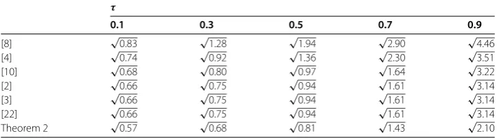
By using the method in Theorem , we list computedr’s for different values ofτ(t) with
μ= in Table . We can see that bounds computed in this paper are tighter than those of references [–, , , ]. Of course, it decreases the conservatism of systems.
Example Consider the following uncertain delayed system:
A+A=
– –.
, A+A=
– –.
, D+D=
– – –.
,
D+D=
– – –.
, B+B=
–.
=B+B, wT(t)w(t)≤,
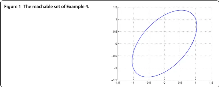
[image:11.595.136.472.311.416.2]Figure 1 The reachable set of Example 4.
and time delay .≤τ(t)≤.,μ= .. The reachable set of system () is plotted in Figure withP=
. –. –. .
.
Remark In the reference [], Domoshnitsky discussed the stability of more
compli-cated linear neutral systems with uncertain coefficients and uncertain delays. In further work, we will study reachable set bounding for this type of linear neutral systems.
5 Conclusions
Firstly, we study uncertain linear systems with polytopic parameters. By using L-K func-tional and novel inequalities to estimate integral terms in L-K funcfunc-tional, some novel suf-ficient conditions for a bounded reachable set of uncertain systems are obtained. Then, we use some examples to show that our methods in Theorems and are effective and have less conservatism compared with reported conditions. Furthermore, the method in this work may be extended to compute a reachable set of linear neutral systems, and it may even be used to deal with stability of linear systems and non-linear systems in the future.
Acknowledgements
This work was supported by the Natural Science Foundation of the Anhui Higher Education Institutions of China (Nos. KJ2016A625, KJ2016A555), the National Natural Science Foundation of China (Nos. 61603272, 11526149), the Youth Fund Project of Tianjin Natural Science Foundation (No. 16JCQNJC03900).
Competing interests
The authors declare that they have no competing interests.
Authors’ contributions
All authors contributed equally to the manuscript, read and approved the final manuscript.
Publisher’s Note
Springer Nature remains neutral with regard to jurisdictional claims in published maps and institutional affiliations.
Received: 13 February 2017 Accepted: 24 October 2017 References
1. Zuo, ZQ, Chen, YP, Wang, YJ, Ho, DWC, Chen, MZQ, Li, HC: A note on reachable set bounding for delayed systems with polytopic uncertainties. J. Franklin Inst.350, 1827-1835 (2013)
2. That, ND, Nam, PT, Ha, QP: Reachable set bounding for linear discrete-time systems with delays and bounded disturbances. J. Optim. Theory Appl.157, 96-107 (2013)
3. Hien, LV, Trinh, HM: A new approach to state bounding for linear time-varying systems with delays and bounded disturbances. Automatica50, 1735-1738 (2014)
4. Zuo, ZQ, Chen, YP, Wang, YJ: New criteria of reachable set estimation for time delay systems subject to polytopic uncertainties. In: The 7th IFAC Symposium on Robust Control Design, Denmark, June 2012, pp. 231-235 (2012) 5. Boyd, S, El Ghaoui, L, Feron, E, Balakrishnan, V: Linear Matrix Inequalities in Systems and Control Theory. SIAM,
6. Tian, JK, Zhong, SM, Wang, Y: Improved exponential stability criteria for neural networks with time-varying delays. Neurocomputing97, 164-173 (2012)
7. Lee, WI, Lee, SY, Par, P: Improved criteria on robust stability andh∞performance for linear systems with interval time-varying delays via new triple integral functionals. Appl. Math. Comput.243, 570-577 (2014)
8. Cheng, J, Zhong, S, Zhong, Q, Zhu, H, Du, Y: Finite-time boundedness of state estimation for neural networks with time-varying delays. Neurocomputing129, 257-264 (2014)
9. Gu, KQ: An integral inequality in the stability problem of time-delay systems. In: Proceedings of the 39th IEEE Conference on Decision and Control, Sydney, December 2000, pp. 2805-2810 (2000)
10. Sun, J, Liu, GP, Chen, J: Improved delay-range-dependent stability criteria for linear systems with time-varying delays. Automatica46, 466-470 (2010)
11. Wu, ZG, Dong, SL, Shi, P: Fuzzy-model-based nonfragile guaranteed cost control of nonlinear Markov jump systems. IEEE Trans. Syst. Man Cybern. Syst. (2017). doi:10.1109/TSMC.2017.2675943
12. Wu, ZG, Shi, P, Su, HY, Jian, C: Sampled-data fuzzy control of chaotic systems based on t-s fuzzy model. IEEE Trans. Fuzzy Syst.22, 153-163 (2014)
13. Wu, ZG, Shi, P, Su, HY, Jian, C: Sampled-data synchronization of chaotic Lur’e systems with time delays. IEEE Trans. Neural Netw. Learn. Syst.24, 410-421 (2013)
14. Wu, ZG, Shi, P, Su, HY, Jian, C: Dissipativity analysis for discrete-time stochastic neural networks with time-varying delays. IEEE Trans. Neural Netw. Learn. Syst.24, 345-355 (2013)
15. Wu, ZG, Shi, P, Su, HY, Jian, C: Reliableh–∞control for discrete-time fuzzy systems with infinite-distributed delay. IEEE Trans. Fuzzy Syst.20, 22-31 (2012)
16. Azbelev, NV, Maksimov, VP, Rakhmatullina, LF: Introduction to Theory of Linear Functional Differential Equations. Advances Series in Mathematical Science and Engineering. World Federation Publishers Company, Atlanta (1995) 17. Azbelev, NV, Maksimov, VP, Rakhmatullina, LF: Introduction to Theory of Linear Functional Differential Equations:
Methods and Applications. Hindawi Publishing Corporation, New York (2007)
18. Azbelev, NV, Simonov, PM: Stability of Differential Equations with Aftereffects: Stability Control Theory Methods and Applications. Taylor & Francis, London (2003)
19. Simonov, PM: To a question on the stability of linear hybrid functional differential systems with aftereffect. Differ. Equ. Qual.2015, 136 (2015)
20. Chudinov, KM: Functional differential inequalities and estimation of the Cauchy function of an equation with aftereffect. Russ. Math.58, 44-51 (2014)
21. Fridman, E, Shaked, J: On reachable sets for linear systems with delay and bounded peak inputs. Automatica39, 2005-2010 (2003)
22. Kim, JH: Improved ellipsoidal bound of reachable sets for time-delayed linear systems with disturbances. Automatica
44, 2940-2943 (2008)
23. Nam, PH, Pathirana, PN: Further result on reachable set bounding for linear uncertain polytopic systems with interval time-varying delays. Automatica47, 1838-1841 (2011)
24. Zuo, ZQ, Wang, ZQ, Chen, YP, Wang, YJ: A non-ellipsoidal reachable set estimation for uncertain neural networks with time-varying delay. Commun. Nonlinear Sci. Numer. Simul.19, 1097-1106 (2014)
25. Park, PG, Lee, WI, Lee, SY: Auxiliary function-based integral inequalities for quadratic functions and their applications to time-delay systems. J. Franklin Inst.352, 1378-1396 (2015)
26. Rugh, WJ: Linear System Theory. Prentice Hall, Upper Saddle River (1996)
27. Zuo, ZQ, Ho, DWC, Wang, YJ: Reachable set bounding for delayed systems with polytopic uncertainties: the maximal Lyapunov-Krasovskii functional approach. Automatica46, 949-952 (2010)
28. Kwon, OM, Lee, SM, Park, JH: On reachable set bounding of uncertain dynamic systems with time-varying delays and disturbances. Inf. Sci.181, 3735-3748 (2011)
29. Domoshnitsky, A, Gitman, M, Shklyar, R: Stability and estimate of solution to uncertain neutral delay systems. Bound. Value Probl.2014, 55 (2014)
30. Agarwal, RP, Domoshnitsky, A, Maghakyan, A: On exponential stability of second order delay differential equations. Czechoslov. Math. J.65, 1047-1068 (2015)
31. Domoshnitsky, A, Maghakyan, A, Berezansky, L: W-transform for exponential stability of second order delay differential equations without damping terms. J. Inequal. Appl.2017, 20 (2017)
32. Domoshnitsky, A, Volinsky, I: About positivity of Green’s functions for nonlocal boundary value problems with impulsive delay equations. Sci. World J.2014, 1-13 (2014)