Predicting Boundary Layer Transition on X 51A Forebody with kT kL (omega) Transition Model

2018 International Conference on Applied Mechanics, Mathematics, Modeling and Simulation (AMMMS 2018) ISBN: 978-1-60595-589-6

Predicting Boundary Layer Transition on X-51A Forebody with kT-kL-



Transition Model

Yu-pei QIN and Chao YAN

Beihang University, Beijing, 100191, China

*Corresponding author

Keywords: Hypersonic, Boundary Layer, Transition.

Abstract. Boundary layer transition is of significance to the hypersonic aircrafts. In this paper, boundary layer transition on X-51A forebody is predicted with the kT-kL-transition model. An overview of the transition zone is depicted and the transition onset on the leeward is compared with the experiment result. The comparison demonstrates that for the complex hypersonic aircraft X-51A forebody, the kT-kL-transition model can reflect the effect of freestream Reynolds number on boundary layer transition, but under certain condition, there is still room to improve the accuracy of boundary layer transition onset prediction.

Introduction

Boundary layer transition from laminar to turbulent flow is always accompanied by a remarkable increase of frictional drag and aeroheating. So it is of vital importance to predict boundary layer transition accurately in a variety of applications, especially for hypersonic aircrafts.

Up to now, boundary layer transition prediction methods include high-precision numerical simulations, such as direct numerical simulation (DNS) [1] and large eddy simulation (LES) [2], nonlinear parabolized stability equations (NPSE) [3], eN [4] method based on linear stability theory and Reynolds averaged Navier-Stokes (RANS) approaches. Transition models based on RANS equations provide a reasonable compromise between accuracy and computational consumption, and become the most practical methods for boundary layer prediction in the engineering level.

To be reliable for a broad range of conditions, flow mechanisms based transition models are more favorable because the transition mechanisms are taken into account directly instead of using transition estimation correlations. In 2008, Walters and Cokjat [5] proposed the phenomenological kT-kL- transition model with the ability to describe the development of the low-frequency velocity fluctuations in the pre-transitional boundary layers. Based on stability theory, Qin et al [6,7] introduce the influence of unstable modes in hypersonic boundary layers and extend the kT-kL-transition model to be appropriate for hypersonic flows. For flat plate and straight cone test cases, results predicted by the revised transition model present good correspondence with the experiment result.

To test the performance of the kT-kL-transition model for the boundary layer prediction of hypersonic complex aircraft, boundary layer transition on X-51A forebody is conducted in this paper.

kT-kL- Transition Model Formation

The revised kT-kL-transition model developed by Qin et al [6,7] is adopted. The governing equations include three transport equations which are the equation for turbulent kinetic energy kT, the equation for laminar kinetic energy kL and the equation for the specific turbulence dissipation rate :

 

_

_

T

T T T

k BP NAT T T

j k j

D k k

P R R k D

Dt x x

 _{  } 



    

     _   _ 

  

 

_

_

L

L L

k BP NAT L

j j

D k k

P R R D

Dt x x



   

      

 _  _ (2)

  _{ } 2

1 2 2 3 3 1 T R

k BP NAT

T W T

T T

T W

j j

D C

C P R R C

Dt k f k

k C f f

x x d        _   _                          _   _         (3)

kT-kL-transition model computes the small-scale viscosity T,s and large-scale eddy viscosity T,l,separately.





, int min , 1 2 , , ,

T s f f kT a kT F T l C k L T l

   _   _    (4)

 is the intermittency factor:

min max kT 1, 0 ,1

C           _  _  _{ }    (5)

 is the boundary layer thickness obtained by the grid-reorder method proposed by Hao et al [8]. The characteristic timescale T,l describes the unstable modes in hypersonic flows.

1 , 1 2 , 1 , 1 nt rel T l

nt nt rel

Ma Ma          _{ }

 (6)

where nt1 and nt2 denote the characteristic timescales of the first and second unstable mode disturbances, expressed as

 

1 1 2 2 2 2

nt Cl eff E uu nt Cl eff U ys

  _ _   _  _

  ， (7)

The local relative Mach number Marel in Eq. 6 is used to demarcate the affected region of different unstable modes. And the effective turbulence length scale eff in Eq. 7 is constructed to reflect the kinematic wall effect.

  2

min , , T

eff nt T T nt

k d U       

  ，  (8)

RNAT and RBP with opposite signs in the transport equations for kT and kL, describe a transfer of energy from laminar kinetic energy to turbulent kinetic energy, and implies the transition mechanism from laminar to turbulent flow.

, /

BP R BP L W NAT R NAT NAT L

R C  k f ，R C  k  (9) Finally, the intermittency factor weighted sum of the large-scale and small-scale viscosities contribute to the RANS equations.

1  ,l ,

T T T s

Test Case

Borg and Schneider [9] has conducted a series of boundary layer transition experiments on the 20% scale X-51A configuration with a full length of 344.2mm. The same model is adopted as Borg’s experiment. A multi-block structured grid is used for calculation. The flow conditions are listed in Table 1.

Table 1. Flow conditions of X-51 forebody.

Ma∞ T0(K) P0(kPa) Re∞ (/m) Tu∞(%) Tw(k) a(°)

Case1 6 428 275 3.2×106 0.36 300 4

Case2 6 428 667 7.8×106 0.36 300 4

Case3 6 428 995 11.7×106 0.36 300 4

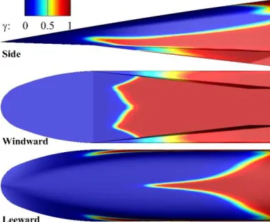
Figure 1 presents the computed transition zone distribution on X-51A forebody when Re∞=11.7×

106/m. It’s obvious that boundary layer transition takes place very forward on the side, which is maybe under the influence of separation and crossflow. On the windward, boundary layer transition occurs on the compression ramp and the transition onset presents in “M” shape. On the leeward, transition zone is mainly concentrated near the centerline and extends to the side as the flow develops downstream.

Figure 1. Transition zone distribution on X-51A forebody (Re∞=11.7×106/m).

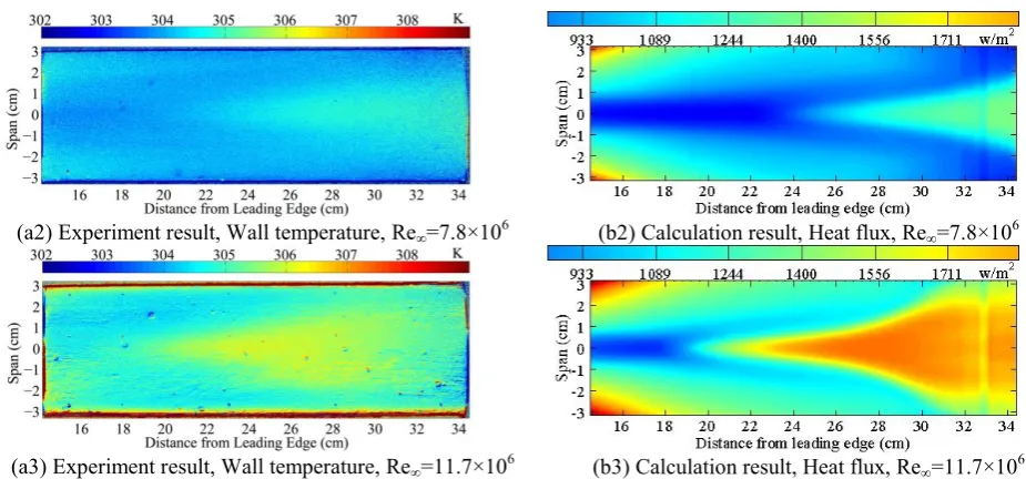
Figure 2 shows the comparison of transition onsets between Borg’s experimental result [9] and the computed results. It’s obvious that when Re∞=3.2×106, both the experimental result and the computed result show that the flow keeps in a laminar state. When Re∞ increases to 7.8×106 and 11.7×106, boundary layer transition takes place on the leeward. The regions where wall temperature increases in the experiment result Figure 2 (a2) and (a3) consist with the regions where the heat flux increases in the computed result Figure 2 (b2) and (b3). Transition onsets of the experimental result present in a “” shape, and the transition onset shapes predicted by the kT-kL- transition model is in good consistency with the experimental result. Besides, as Re∞ increases, the computed transition onset moves forward, which agrees well with the experimental result and stability theory. Such a phenomenon can demonstrate that the kT-kL- transition model can reflect the influence of Reynolds numbers on boundary layer transition properly.

(a2) Experiment result, Wall temperature, Re∞=7.8×106 (b2) Calculation result, Heat flux, Re∞=7.8×106

(a3) Experiment result, Wall temperature, Re∞=11.7×106 (b3) Calculation result, Heat flux, Re∞=11.7×106

Figure 2. Comparison of transition onsets under different freestream Reynolds numbers.

To validate the prediction accuracy of the kT-kL- transition model, the computed heat flux distribution along leeward centerline are compared with the temperature distribution along leeward centerline by the experiment [9] in Figure 3. If the position where the wall temperature and heat flux begin to increase is defined as the transition onset, when Re∞=3.2×106, there are not transition process for both the experimental result and the computed result. When Re∞=7.8×106, transition onset of the

experimental result is at x≈16.3cm. While there is an obvious delay for the computed transition onset

which is at x≈21.4cm. When Re∞=11.7×106, the experimental transition onset is at x≈15.3cm, and

the calculation result is at x≈17.0cm. For this condition, the computed transition onset agrees well

with the experimental result. Besides, the position where the maximum heat flux occurs (x≈27.1cm)

shows discrepancy with the experimental result where the maximum wall temperature presents (x≈

23.6cm).

(a) Temperature distribution along leeward centerline, Experiment result

(b) Heat flux distribution along leeward centerline, Calculation result

Figure 3. Comparison of transition onsets on the leeward centerline.

Summary

(1) For the complex hypersonic X-51A forebody, the kT-kL-transition model can reflect the influence of the freestream Reynolds number on the boundary layer transition. As Re∞ increases, boundary layer transition onset delays.

(2) The kT-kL-transition model can predict the same transition onset shape as the experimental result, but for transition onset positions, under certain condition, there is a remarkble discrepancy between the computed result and the experimental result.

(3) On the side of X-51A forebody, boundary layer transition takes place much forward than the windward and leeward, which needs further investigation.

References

[1] C. Liu, P. Lu, DNS study on physics of late boundary layer transition, AIAA Paper, 2012, AIAA-2012-0083.

[2] R. Bouffanais, Advances and challenges of applied large-eddy simulation, Comput. Fluids 39(5)(2010) 735-738.

[3] T. Herbert, Parabolized stability equations, Annu. Rev. Fluid Mech. 29(1)(1994) 245-283.

[4] J. L. van Ingen, The eN method for transition prediction, Historical review of work at TU Delft, AIAA Paper, 2008, AIAA-2008-3830.

[5] D.K. Walters, D. Cokljat. A Three-Equation Eddy-Viscosity Model for Reynolds-Averaged Navier-Stokes Simulations of Transitional Flow, Journal of Fluids Engineering, 130 (12) (2008):320-327.

[6] Y.P. Qin, C. Yan, Z.H. Hao, L. Zhou, A laminar kinetic energy transition model appropriate for hypersonic flow heat transfer, International Journal of Heat and Mass Transfer, 107 (2017) 1054-1064.

[7] Y.P. Qin, C. Yan, Z.H. Hao, J.J. Wang, An intermittency factor weighted laminar kinetic energy transition model for heat transfer overshoot prediction, International Journal of Heat and Mass Transfer, 117 (2018) 1115-1124.

[8] Z.H. Hao, C. Yan, L. Zhou, Y.P. Qin, Development of a boundary layer parameters identification method for transition prediction with complex grids, J. Aerosp. Eng., 231(11)(2017) 2068-2084.